Within Excel there is not a single formula to get the last element within a column or a row, but it can be achieved by a combination of worksheet functions within a variety of differing requirements. The fact that this is achieved in Excel by combining a number of functions can be seen as a strength of Excel (a strong base set of functions that provide a large degree of extensibility), or a weakness (lack of commonly required functions), depending upon your viewpoint.
The following is an extract of a comprehensive White Paper Bob Phillips and I created together. If you want more details about getting the last value including alternative solutions, benchmarks, VBA coding, etc. you may take a look at it.
- Getting the last numeric value in a column:
- Formula: =INDEX(A:A,MATCH(9.99999999999999E307,A:A))
- The INDEX/MATCH formula searches for the value 9.99999999999999E307. This value is the highest value that can be represented in Excel. Therefore this formula returns the last numeric value that is smaller than or equal to this number.
- If no numeric entry exists within the range, the MATCH formula will return the #N/A error.
- Getting the last text value in a column:
- Formula: =INDEX(A:A,MATCH(REPT(“Z”,255),A:A))
- The INDEX/MATCH formula uses a string consisting of 255 ‘Z’ characters to find the last text entry. For Excel, this string evaluates to the ‘largest’ string value.
- You cannot use the function REPT(CHAR(255),255), as the largest value. Whilst you might suspect that Excel evaluates this to the ‘largest’ string value, Excel evaluates the following formula:
=REPT(“Z”,255)<rept (CHAR(255),255)
to FALSE - Getting the last value of any type in a column:
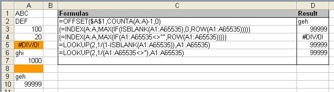
- Formula: =LOOKUP(2,1/(1-ISBLANK(A1:A65535)),A1:A65535)
- This formula uses LOOKUP in its vector syntax form, with the lookup value as the first parameter, the lookup vector as second, and the result vector as the last parameter.
- The most interesting part of this formula is the lookup vector (the 2nd parameter). The formula element
1/(1-ISBLANK(A1:A65535))
in this example returns the following array
{1;1;1;1;1;1;1;#DIV/0!;1;1;#DIV/0!;#DIV/0!;…;#DIV/0!}
that is, the ISBLANK function returns an array of TRUE (blank cell) or FALSE (non-blank cell) values. Subtracting this from 1 converts the array to an array of 0 (blank) or 1 (non-blank) values. Dividing 1 by this array then returns an array of #DIV/0 (blank) or 1 (non-blank) values. - The LOOKUP searches for the value ‘2’ within the array (which now consists only of ‘1’ and #DIV/0 values). The LOOKUP will not find this value, so it matches the last value that is less than or equal to lookup value. This is the last ‘1’ within the range which represents the last filled cell.
- Restriction: you can’t use a complete column reference such as A:A for this type of formula.
- This type of formula can be used for a lot of similar problems using the second parameter to create a lookup vector consisting of either ‘1’ or ‘#DIV/0’ errors by setting the Boolean expression accordingly. I personally saw this usage first in a posting from Aladin Akyurek.
All these formulas can easily adapted for searching in a row by changing the range reference. For examples see the above mentioned White Paper.
There are some very efficient worksheet functions that find the last row/column (which can either be the last visible row/column containing data or the last used row/column) and return counts of rows/columns available from my website:
http://www.decisionModels.com/downloads.htm
The functions will also handle both rectangular and irregular blocks of data, which can contain mixed alphabetic, numeric, date, time , errors etc
Charles Williams
In #2, you mention that CHAR(255) sorts before “Z”, a.k.a. CHAR(90). If you setup a column of numbers 1-255, and next to that a column of CHAR(A1), CHAR(A2), etc, and then sort on column B, you’ll see why.
Within the letters section, Excel sorts all letters that look similar together. So, for example, U and all of its variants (accented, umlauted, etc) are together. Char(255) is actually a lower-case y-umlaut (at least on my US English PC), and as such sorts before the Z’s.
Incidentally, there are four “Z”‘s showing on my PC – they are ASCII 90 (Z), 122 (z), 142 and 158. So technically, matching against REPT(CHAR(158),255) would be most correct.
Of course, Excel 2003 can contain strings much larger than 255 characters, so method #2 would still have an incorrectly handled edge case if you had a string in the column of, say, 1024 CHAR(158)’s…
Hi Kevin
thanks for your comment. The output though looks a bit different on my (German) Windows PC but you’re correct that CHAR(158) is ‘larger’ than ‘Z’. Lets say
REPT(“Z”,255) should be sufficient for nearly all ‘real-world’ cases :-)
It is unfortunate that people continue to propagate the INDEX(MATCH(9.9999E307… and the corresponding method for text entires as a means to find the location of the last entry in a column.
Two major problems exist with these methods.
First, they are limited to one type of data item and provide incorrect results with mixed data types. Ironically, and as noted in the post by Kevin, the REPT(“Z”…) approach is flawed even when dealing with text values.
Second, they rely on a bug in XL wherein the implementation of various functions, including MATCH, do not match the documentation — or the intent! One hopes that Microsoft will fix its problems even if it hasn’t for a decade or more — if for no other reason than to live up to its own claim of trustworthy computing. When that happens, every solution in the class of INDEX(MATCH(large-number…) will suffer a major case of Humpty Dumpty!
For more, see http://groups.google.com/groups?threadm=MPG.1973429a8eb8e78e98aba5%40msnews.microsoft.com
Even before considering the oneliner VBA function listed in the archived discussion at google groups, consider this:
The norm for a list is to have contiguous entries. In fact, all modern tools for data analysis rely on the underlying data being organized along the rules of relational data bases.
That means that OFFSET(…COUNTA()) will always provide a correct result. If there is a problem in the data structure — holes in a list or multiple lists one below the other or whatever — the solution is not to come up with formulas of ever-increasing complexity, but to fix the problem at the source.
Hi Tushar
I think I disagree slightly with you on that topic :-)
1. As stated the INDEX/MATCH functions work only for one specific data type. If you know your data structure these formulas are much faster than all other solutions.
2. For text values: again it’s not very likely that you have a text entry which is ‘larger’ than REPT(“Z”,255).
3. Re: Documented behaviour: While I agree that the help states a different behaviour I doubt that MS will change this implementation. It would be eaiser just to change the help content ;-)
4. While in most real case scenarios the OFFSET/COUNTA function may work they also depend on one assumption (no blank cells in between).
And as stated in the referred link VBA solutions also have their drawbacks. In the end the user should decide which solution fits best to his requirements and what assumptions he can make.
Frank
Frank –
That’s a fine paper you and Bob put together. Thoughtful, analytical, with actual benchmark studies. I’ll be studying those formulas.
– Jon
Hi Jon
many thanks for your comment. Bob and I are currently working on more of these white papers (we just need more time…)
I’ll post some excerpts on this blog once they’re ready :-)
Frank
Hi Tushar,
My understanding of relational theory is that nulls/blanks are perfectly valid in tables. And all the RDB’s I have ever worked with allow them.
So I do not think it is correct to say that you should always fix the problem at the source by redesigning the data.
Also there is no good theoretical reason to insist on only having one table on a worksheet (in fact doing that generally slows down the Excel calculation engine).
Its not difficult to design UDFs that doe not have these limitations and work faster than COUNTA and the more complex array formulae: see the counting functions at
http://www.decisionModels.com/downloads.htm
for examples.
You’re a lifesaver. One question, though.
What needs to change in the formula if I want to return the value of the last visible cell in a filtered column?
Mr Kabel,
I tried using the formula you placed here, (Formula: =INDEX(A:A,MATCH(9.99999999999999E307,A:A)) ) in a cell on my Excel Sheet.
I always get the Message that ‘the formula you typed contains an error’
What am I doing wrong…
Benoit Houle
atlan@videotron.ca
Don’t put in column A. Also, make sure you have the same number of closing parens as you do open parens. That’s a pretty common cause of the error.
Thanks a lot :>
I would like to know if you have anything that will show only the last number that is greater than “0??
Jess
Thanks, I found the ‘getting the last numeric value in a column’ section extremely helpful. Perhaps this should be added to Excel’s list of functions.
Naomi
Thanks, the lookup formula posted helped me alot. Although I have a question. why is there a 2 in the lookup function? (i.e. -lookup(2,…..)). does it matter? I noticed that any number greater than 0 works?
just a thought
Jaime
Jaime: Actually it does matter. If you change
to
, you’ll see that 1 and 2 as the lookup value give different results. When there are ties, such as a 1 in the lookup value and more than one 1 in the lookup vector, which 1 it returns is unpredictable. However, since 2 will always be greater than anything in this lookup vector, you know it will always return the last 1. Any number above 2 will work exactly the same as 2.
Here’s another formula, just for the record
Thanks for the explanation. it makes more sense now
I’m trying to get the formula to return the second last value (3rd last, 4th last, etc) for any type of value. For numeric values the formula =LOOKUP(9.99999999999999E+307,A1:INDEX(A1:Z1,MATCH(9.99999999999999E+307,A1:Z1)-1)) works.
I have tried =LOOKUP(2,1/(1-ISBLANK(D46:IG46)),D46:INDEX(D46:IG46,LOOKUP(2,1/(1-ISBLANK(D46:IG46)),D46:IG46)-1)), but am getting an error.
Any help would be appriciated.
Thanks for the formula to grab the last text entry in a column, BUT I am also working with a column that is formatted for DATE. Is there a similar function to grab the last date in a cloumn?
Thanks.
hello everyone, trying to move multi lines of almost identical data from one sheet to another sheet for formatting. 1 to 150 lines all identical except purchase qtys and purchase order line number. over 400 part numbers to move. any ideas how to do a vlookup like function on multi lines and multi rows without being stuck using pivot tables?
How can i find the last value in a row that have cells with !N/A#?
Thanks a lot
In #3 above, you can use the formula in C3.
In response to the error returned when you put the numeric formula in its own column.
This can be avoided if you can specify the range of rows you are searching within that column.
Example =INDEX(G2:G39,MATCH(9.99999999999999E+307,G2:G39))
For when you want the result to be in the same column.
I tried the formula to find the last value in a column. Every cell in the column does not have an entry, for example, the column goes from G4:G100 and there are some 30 enttries, however, based on another worksheet that feeds into the G4:G100, the values and location of data change. I still need to find the last numeric value in the “G” Column. When I use the formula above I get a #NULL! result.
thank you for your time and consideration.
I have been trying to use this formula to pull the last text value from a column in a spreadsheet to another spreadsheet, which is my Summary Page.
Is there a specific formula that someone can write out for me that will find the last entered text in a cell within a column in one spreadsheet and show that text in another spreadsheet?
Help! I am not an Excel Guru.
Thanks for your suggestions.