I have these four favorites defined in Outlook:
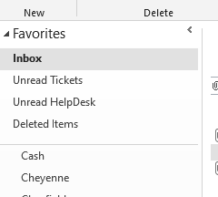
From the inbox, I could hit Shift+F6 to get into the Favorites area but sometimes I would end up in no man’s land and couldn’t figure out how to get back into the inbox. So, god forbid, I had to use my mouse. I wrote this macro:
|
1 2 3 4 5 6 7 8 9 10 11 12 13 14 15 16 17 18 19 20 21 22 23 24 25 |
Sub NavigateFavorites() Dim ae As Explorer Dim oMod As MailModule Dim oGrp As NavigationGroup Dim oFldrs As NavigationFolders Dim i As Long Set ae = Application.ActiveExplorer Set oMod = ae.NavigationPane.Modules.GetNavigationModule(olModuleMail) Set oGrp = oMod.NavigationGroups.GetDefaultNavigationGroup(olFavoriteFoldersGroup) Set oFldrs = oGrp.NavigationFolders For i = 1 To oFldrs.Count If oFldrs(i).DisplayName = ae.CurrentFolder.Name Then If i = oFldrs.Count Then Set ae.CurrentFolder = oFldrs.Item(1).Folder Else Set ae.CurrentFolder = oFldrs.Item(i + 1).Folder End If Exit Sub End If Next i End Sub |
And added it to the fourth position on my QAT. Now I can press Alt+4 to cycle through my favorites. And I’ve only hit Alt+F4 accidentally about a dozen times.