I want to describe for you a process that I do many times every month. Then I’m going to tell you how I tried, and failed, to make it easier. Put on your seat belts, here we go.
I repeatedly have situations where I have two CSV files containing lists. Each list has an Invoice # column and a Sales Dollars column, but there’s not guarantee that they’re actually called by those names. Also, each list has multiple other columns.

There is an inconsistency between these two lists. The total sales for any invoice should be the same no matter how it’s sliced and diced. With this simple example, it’s easy to see that invoice 9452 has problems. With 100 invoices and more than one problem to find, it’s not so easy to do it visually.
My first attempt at this was to combine the two lists, rearranging the columns so that the relevant ones match up, adding a new column to distinguish the lists, and creating a pivot table. If I were to apply that method to this simple example, it might look like this:
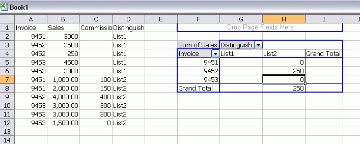
I right-clicked on the Sales field (in the data area) and chose Field Settings and set these options to get the difference
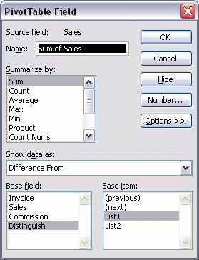
With my sample lists, this isn’t too bad of a method. With the actual data, there are more columns to have to move around and there are total and subtotal rows that muddy things up. It’s still not too bad, but I went to search for something better. My next step, was to make my own pivot table using the SUMIF function. I start by guessing which list has the most complete list of invoice numbers and creating a unique list of invoice numbers from that.
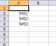
To get that list, I use this macro. Next I create two columns of formulas using SUMIF.
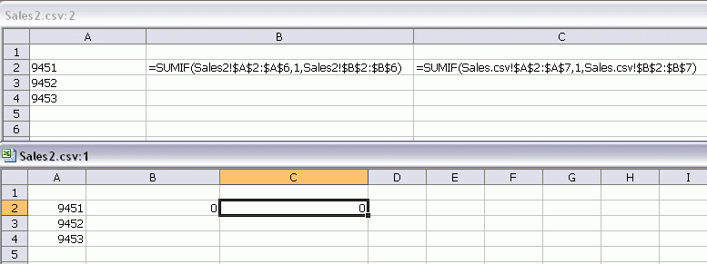
You might notice that the second argument for SUMIF is ‘1’, rather than the cell reference you would expect. The problem with SUMIF is that the first and third arguments are ranges that are on a different page than the second. That means I have to go select the range, then return to the first page to select the criteria, then go back to the second page to select the sum_range. It’s a pain, so I put a ‘1’ as a place holder in the formula, then edit the formula to point to the right range.

I replaced the ‘1’s with a cell reference, copied the formulas down, and created a difference column. Awesome, you say? It’s still pretty cumbersome. The only advantage over the pivot table method is that I can do it all from the keyboard. A point that I will learn is important (to me) later. But it’s still the same amount of manual drudgery as the pivot table method, so I set to automating it.
I started with a simple userform that let me select the pertinent arguments to the SUMIF function.
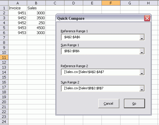
The Go button creates a new sheet, creates a unique list from Reference Range 1 and Reference Range 2, and creates the SUMIF and difference formulas. It basically does what I did manually. I started with RefEdit controls, but switched to PeltierTech’s alternative to RefEdits on this form. Did you know that you can’t use Control+Tab to switch workbooks with a RefEdit?
This method is slightly faster than the manual method, slightly less prone to errors, and ensures that I have complete unique list. Do you know that feeling you get when you automate a piece of drudgery; that uplifting, everything-is-great, top-of-the-world feeling? I didn’t have that feeling as evidenced by how many times I used the word ‘slightly’ when listing the benefits.
Switching workbooks using Control+Tab doesn’t work with the alternative to RefEdit either and it’s the biggest disappointment to me with this method. You likely already know that I’m fanatical about avoiding the mouse, but this isn’t mere fanaticism. Having to use the Window menu to switch workbooks is an acceptable use of the mouse as long as there are benefits to offset my having to reach over. Selecting long ranges with a mouse, however, makes me want to punch myself in the face. That means I have to use my mouse to switch windows, go back to the keyboard to select the range, then back, then forth. Bleh. I made things worse trying to make things better.
I think my next step is to go back to the pivot table method and try to automate that. If I could get the columns lined up properly that would be a good start. Failing that, maybe I can hire someone from a developing country to do the work for me. I’ll send them two CSV files and they can return the pivot table. I’ll pay them $1 per calculation, but it has to be returned in less than 5 minutes. I’ll give them a $1 bonus if they get it back in under a minute. Now that’s an idea with legs.
Here’s the controlling code for the userform:
Dim ufQuick As UQuickCompare
Dim rCell As Range
Dim sFormula As String
Dim colUnique As Collection
Dim ws As Worksheet
Dim i As Long
Set ufQuick = New UQuickCompare
ufQuick.tbxRefRange1.DropButtonStyle = fmDropButtonStyleReduce
ufQuick.tbxRefRange1.ShowDropButtonWhen = fmShowDropButtonWhenAlways
ufQuick.tbxRefRange2.DropButtonStyle = fmDropButtonStyleReduce
ufQuick.tbxRefRange2.ShowDropButtonWhen = fmShowDropButtonWhenAlways
ufQuick.tbxSumRange1.DropButtonStyle = fmDropButtonStyleReduce
ufQuick.tbxSumRange1.ShowDropButtonWhen = fmShowDropButtonWhenAlways
ufQuick.tbxSumRange2.DropButtonStyle = fmDropButtonStyleReduce
ufQuick.tbxSumRange2.ShowDropButtonWhen = fmShowDropButtonWhenAlways
ufQuick.Show
With ufQuick
If Not .UserCancel Then
Set colUnique = New Collection
For Each rCell In .RefRange1
On Error Resume Next
colUnique.Add rCell.Value, rCell.Text
On Error GoTo 0
Next rCell
For Each rCell In .RefRange2.Cells
On Error Resume Next
colUnique.Add rCell.Value, rCell.Text
On Error GoTo 0
Next rCell
Set ws = ActiveWorkbook.Worksheets.Add(ActiveSheet)
For i = 1 To colUnique.Count
ws.Cells(i, 1).Value = colUnique.Item(i)
ws.Cells(i, 2).Formula = “=SUMIF(” & .RefRange1.Address(, , , True) & _
“,” & ws.Cells(i, 1).Address(0, 0) & “,” & .SumRange1.Address(, , , True) & “)”
ws.Cells(i, 3).Formula = “=SUMIF(” & .RefRange2.Address(, , , True) & _
“,” & ws.Cells(i, 1).Address(0, 0) & “,” & .SumRange2.Address(, , , True) & “)”
ws.Cells(i, 4).FormulaR1C1 = “=RC[-2]-RC[-1]”
Next i
End If
End With
Unload ufQuick
Set ufQuick = Nothing
End Sub
![]() You can download QuickCompare.zip
You can download QuickCompare.zip
Hi Dick
I’m not sure if this is any help, but there used to be a excel add-on floating about the web that was great for reconciling data. It’s a long time since I used it. I was by BlackIron Financial and the file was xlwzrecon.xla. Might be useful to someone.
Best wishes
Martin
Okay, so maybe I totally and completely missed something, but if you want to do this type and data scrubbing/analysis, why not use SQL? Why not set up the sheets as data sources and write SQL statements that do all this heavy lifting for you?
Granted, it will take some time to do the initial set-up, write the SQL, and put in place, but once there, you should only have to be checking that the columns in question retain the names you need for the SQL to work month in and month out.
Or, like I said, maybe I missed something?
I would use a virtual array combined with a dictionary lookup.
Load the first list into a virtual array arINP1.
As you process each invoice no. in arINP1, you use the dictionary lookup to check whether you have encountered that invoice before.
If NOT, increase an output row count and save this against the invoice number in the dictionary. Then save the data at that row position into a virtual array arOUT.
If SO, the dictionary returns the row number in the virtual output array arOUT. You then add the data from arINP1 to the relevant row in arOUT.
Then load the second list into arINP2 and use the same dictionary as you process each invoice in that array, adding the data into a separate column of arOUT.
Finally calculate differences in a third column and then save the arOUT onto a worksheet.
I think you get the idea.
ScottL: The column headings are unpredictable, so I think I’d have to change the SQL every time.
“The column headings are unpredictable…”
Can they not be changed, once you have the CSV files in your possession?
Yep, I can change the column headings. But I don’t think that actually saves me time.
Have you tried creating a Lookup() or vLookup() function to draw the values from one list into a column of your choice? Then you can use a formula to note the difference, if any, between one list and the other.
Dick: I’m not suggesting that one solution is better than the other, but regarding the column headings, just how many columns are you dealing with here? How unpredictable are they (i.e., are they “Name”, “Rank”, “Serial Number” one month, and “Lastname”, Organizational Position”, and “Soldier ID” in the next)? Is it something you can (again, time spent up front), can code for all the potential variables, then run a routine that cleanses the headings?
I guess what I’m trying to say is that, if the data itself is good, I wouldn’t let crappy field headings completely submarine a potential solution. The data is so much more important than how it’s labeled…
Again, not saying one is better than the other, just trying to understand how difficult the headings are…
You can do this using dynamic ranges and array formulae. It’s a bit cumbersome to set up, but the idea is that you copy and paste one csv file into a worksheet called List1, and the other into a worksheet called List2.
Set up another worksheet called Ranges: this is to make named ranges formulae more readable. In it you have named cells called InvColList1, which has the column letter for the invoice numbers in List1, and similarly InvColList2, SalesColList1 and SalesColList2.
Then set up named cells called InvCountList1, which contains the formula
=COUNTA(INDIRECT(“List1!$”&List1InvCol&”:$”&List1InvCol)
This counts the non-blank cells in the column with the invoice numbers in List1
Do similar named cells called InvCountList2, SalesCountList1 and SalesCountList2. You don’t really need the SalesCount variables, but it’s a good visual check that they’re the same numbers as the InvoiceCount variables, as I suspect things would go a little haywire if there are differences.
Then set up dynamic named ranges for the invoice numbers and sales amounts – the formulae in the name manager are:
InvoiceList1=OFFSET(INDIRECT(“List1!”&List1InvCol&”2?), 0, 0, List1InvCount-1, 1)
InvoiceList2=OFFSET(INDIRECT(“List2!”&List2InvCol&”2?), 0, 0,List2InvCount-1, 1)
SalesList1=OFFSET(INDIRECT(“List1!”&List1SalesCol&”2?), 0, 0, List1SalesCount-1, 1)
SalesList2=OFFSET(INDIRECT(“List2!”&List2SalesCol&”2?), 0, 0,List2SalesCount-1, 1)
All this is a bit of a pain, but it means that you don’t have to anything else next time apart from paste the csv files in, and update the column letters.
The final step is to put in a results worksheet, with columns headed Invoice Number, Sales1 Price, Sales2 Price and Discrepancy, in columns A to D respectively.
In cell a2, put the formula
=IFERROR(IFERROR(INDEX(InvoiceList1,MATCH(0,COUNTIF($A$1:A2,InvoiceList1),0)),INDEX(InvoiceList2,MATCH(0,COUNTIF($A$1:A2,InvoiceList2),0))), “”) and hit Control+Shift+Enter
This array formula I adapted from here: http://www.get-digital-help.com/2009/06/16/extract-an-unique-distinct-list-from-two-columns-using-excel-2007-array-formula/
In b2, enter =SUMIF(InvoiceList1, A2, SalesList1)
In c2 enter =SUMIF(InvoiceList2, A2, SalesList2)
and in d2 enter =IF(B2=C2, “”, “Error”)
Then all you need to do is put in a filter, and select the rows where column d is “Error”.
If anyone wants a copy of the spreadsheet (it’s Excel 2007), post a comment and I’ll send it along.
You’re right ScottL. I could hard code three column names per column and get 98% of the situations, I just wanted something more general purpose. It’s a balance, I think, determining how general to make a solution when a specific solution could be done quickly and easily.
This sounds like a job for SQL.
In an Access database, create lista and listb tables, then run the following sql:
select invoice, sales_a, sales_b, sales_a – sales_b as diff from
(select x.invoice, (select sum(sales) from lista where invoice = x.invoice) as sales_a, (select sum(sales) from listb where invoice = x.invoice) as sales_b
from (select invoice from (select invoice from lista union select invoice from listb) group by invoice) x)
Rob: You and I are on the same page, it’s just a matter of where to run the SQL itself. But Dick raises a really interesting point. Originally he was walking through the process he tried for his own problem, and how it did (or didn’t really) work. Later though, after a number of good and varied suggestions, he commented that he was hoping to come up with a more generic solution that could be applied without a lot of personal customization (presumably so he could easily re-use it or so that the readers here could adapt it if necessary).
So I guess my question is this, and I guess it’s for Dick: are you looking for feedback on how to solve your problem specifically, or are you looking for how Average Joe might tackle the problem without too much custom tweaking?
(Then again, given the blog as a whole and comments on the blog, I’m thinking there aren’t as many “Average” Excel users browsing these types of topics… :-) )
Another vote for SQL here.
Why not have a utility that opens the CSV, reads off the column headings so that it can build the queries correctly, closes it then connects via ADO and then gets the data that way?
This would get round the changing nature of the headings.
Field names may change, but do field positions? If field positions are always the same, a fairly straightforward batch file could replace random field names with specific, invariant field names.
@echo off
if “%1? == “” (echo usage: %0 CSV_filename & goto :EOF)
echo IDSalesFld3Fld4 . . . > “rev.%~1?
for /F “usebackq skip=1 tokens=*” %%a in (“%~1?) do echo %a >> “rev.%~1?
Then it should be possible to use a canned SQL procedure to process the rev.filename.csv files. Even if the Invoice ID and sales fields are in different positions, it’d still be possible to import the CSV files into different worksheets in an Excel workbook, name the invoice ID and sales fields, save the workbook, then link to those worksheets in Access using specific names, and run canned queries against those tables.
Always use the best tool for the task, and in this case Access/SQL is much, much better than anything you could come up with in Excel, no matter how clever.
No solution suggestion; just an observation. The real question is why the heck do you have data sets that have different sales numbers. Some really old accountants are rolling over in their graves right now :)
are you looking for feedback on how to solve your problem specifically Not necessarily, but any comments are appreciated.
why the heck do you have data sets that have different sales numbers The real reason is that one of the data sets is Quickbooks, so I have to do in Excel what QB won’t do. We can’t all afford enterprise software. :)
hi fzz
regarding “Always use the best tool for the task, and in this case Access/SQL is much, much better than anything you could come up with in Excel, no matter how clever.”
AFAIK the same queries can be run from Excel as from Access. Just connect to the data and execute the query. The approach is virtually identical. Am I missing something?
regards, Pete
Always use the best tool for the task, and in this case Access/SQL is much, much better than anything you could come up with in Excel, no matter how clever.
If both Excel and Access produce the same result, how is one better than the other? In terms of ease of maintenance, that would be a matter of opinion.
Rob: I’m guessing that what fzz means (fzz: don’t mind if I put words in your mouth) is that, in Access, setting up two tables and quickly querying them is a pretty simple straightforward procedure. Sure, the same thing can be done in Excel, but you’re writing the SQL yourself, and, if using Extended Properties=Excel 8.0, then you have to be careful with the table names (using “$”, etc.). Access just makes all that easier.
That said, I’d love to see an Excel app that does all that for you. Something to ponder building in the future…
Each method has its merits, sql wins in scalability and performance but imho it’s hard to beat the flexibility of the pivottable.
I’d group and hide matching rows then drill down on subtotals and use the extra column to annotate the differences. One way to do this is select the data range row differences with ctr+ ” then group selected invoice numbers by pressing Alt+;.
To create the pivot directly, either use a union query or multiple consolidation ranges eg:
sendkeys “~i~”: application.Dialogs(xlDialogPivotTableWizard).Show 3, [{“sheet1!r1c1:r6c2″,”1″;”sheet2!r1c1:r7c3″,”2”}]
[…] June 9, 2010 at 5:26 PM | Posted in General | Leave a Comment Tags: aggregated, compare Dick describes a situation where he has two lists of invoices. In each list, the invoices are separated into rows according to […]
I came across the site today, and you helped me solve a problem with carriage breaks from text I was querying from a SQL Server. Thanks!
My recommendation for this problem is to connect to the CSV file through data connectivity. Data – Get External Data – From Text. Setup your pivot table like you did before. Save your file. Next month, save your CSV file in the same location, with the same name. Then all you have to do is allow data connectivity to update the data when you open the workbook with the PivotTable. Refresh your PivotTable, save your file with the new month, and you are done. When you set up your PivotTable, just make sure the source data is not a set array. It should default to something like Sheet1!CSV.
That’s seems like the most efficient method to me.