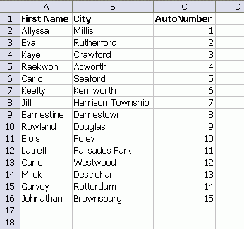
Here are three ways to lookup a value based on two columns. Let’s start with this random data:

And let’s say that we want to lookup the autonumber value for Carlo. Not the Carlo in Seaford, but the Carlo in Westwood.
SUMPRODUCT
With ‘Carlo’ in E2 and ‘Westwood’ in F2, use =SUMPRODUCT(($A$2:$A$16=E2)*($B$2:$B$16=F2)*(C2:C16))
If you have more than one Carlo/Westwood combination, you’ll get the sum of all of them. One advantage of this method is that you don’t need any helper columns. If you can’t mess with your data, it’s a good option. However, if you have a lot of these formulas, it can become slow.
VLOOKUP
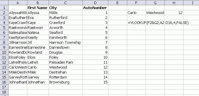
To use VLOOKUP, we’ll need to add a column on the left. VLOOKUP only works when the look up column is the first column. In the new column A, I concatenated columns B and C.

=VLOOKUP(F2&G2,A2:D16,4,FALSE)
This is quicker than SUMPRODUCT, but you won’t see the difference until you have a lot of formulas. The downside, obviously, is that you have to add another column on the left.
INDEX
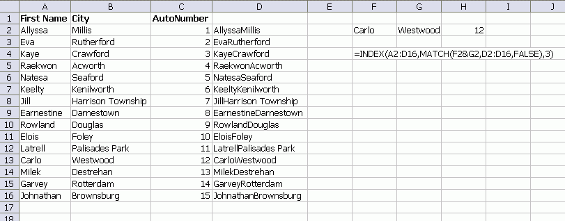
For the INDEX method, you still have to add a new column, but it doesn’t have to be the first column.

=INDEX(A2:D16,MATCH(F2&G2,D2:D16,FALSE),3)
Same benefits and detriments as the VLOOKUP option, but you can tack that extra column on the end.
You can also use:
INDEX($A$2:$D$16,MATCH(1,(F2=$A$2:$A$16)*(G2=$B$2:$B$16),0))
You need to enter it as an array formula. It’s similar in nature to the sumproduct, but sumproduct doesn’t work if the figure that you’re trying to look up isn’t a number.
Quibble: concatenating fields without explicit field separators can occasionally lead to unexpected (wrong) results.
There’s no need for string concatenation, which is usually slow. Use an array formula.
=INDEX(A2:C16,MATCH(TRUE,IF(B2:B16=G2,A2:A16=F2),0),3)
Or if the last match is as good as the first match, use the regular formula
=LOOKUP(2,1/(B2:B16=G2)/(A2:A16=F2),C2:C16)
Although slower, the SUMPRODUCT approach allows a few other advantages:
– Greater flexibility in the number and variety of criteria you can use in selection; the VLOOKUP/INDEX approach can get messy if you have 5 different combinations of data that you need for selections
– The SUMPRODUCT approach can provide both SUMIF and COUNTIF functionality that the VLOOKUP/INDEX approaches do not
The glaring problem is that sumproduct will only return results if you are looking up a numeric value. If column C in your first example had alphanumeric data (as you might want from a vlookup), it would give you a #VALUE!.
I don’t have a solution to that.
But if you are looking at just numbers and have XL07, I recommend the new SUMIFS formula. It is dramatically faster than using SUMPRODUCT or an array formula.
Treat the table as the source for a SQL query.
All good points. I need a pipe seperater in there.
Tushar: I’ve done it, but I don’t trust it. I trust the results, but it seems like it could break at any minute. Has anybody done any good testing on it?
Dick: I have used SQL queries for “production” systems. The Excel worksheets have had several thousand rows of data and some queries included joins across tables in different worksheets.
I have also queried data in corporate databases to extract the data into Excel.
What I sometimes do is use the query for the initial analysis, then use that as the source for further analysis, which might be some kind of “roll your own” result or a PivotTable or Chart.
I have had no problems with this approach.
You can use a SUMPRODUCT to return a text result from a Multi-criteria lookup. Someone asked me for a multicriteria vlookup here it is
=INDEX(C2:C7,SUMPRODUCT(MATCH(TRUE,(A2:A7&B2:B7)=(F2&G2),0)),1)
It finds the first instance only. I had never used a MATCH within a SUMPRODUCT, but it seems to work ok.
Another example of the flexibility of the humble SUMPRODUCT function.
You could also use a combination of INDEX and MATCH without a helper column. Needs to be array-entered:
=INDEX(C2:C16,MATCH($E$2&”|”&$F$2,$A$2:$A$16&”|”&$B$2:$B$16,0))
I used SQL queries a lot in certain Excel models, with success. Officialy, it’s documented as a technology to use on closed workbooks, but it works fine on open workbooks. It does give me sometimes an I/O error when closing the file after debugging. But it works like a charm in production.
i like this rray formula:
=INDEX($C$2:$C$16, MATCH(1, ($A$2:$A$16 = F2) * ($B$2:$B$16 = G2), 0))
If you use Excel 2007, then you can convert the range into a Table, and the array formula looks nicer, and grows without fancy dynamic ranges:
=INDEX(Table1[AutoNumber], MATCH(1, (Table1[First Name] = F2) * (Table1[City] = G2), 0))
In the past I was a power user of SQL & Excel Workbooks. However, after having some seriously issues with memory leak with one client’s solution I now use it less.
Kind regards,
Dennis
If you know the list to be unique and you’re still looking up a number, you could use SUMIFS or AVERAGEIFS in 2007. On a table, the formula would be:
=SUMIFS(tbl[AutoNumber],tbl[First Name],F2,tbl[City],G2)
Very readable and much faster than SUMPRODUCT.
To avoid the CSE.
=INDEX($C$2:$C$16, MATCH(1, INDEX(($A$2:$A$16 = F2) * ($B$2:$B$16 = G2),0), 0))
Regards
Interesting question whether both ($A$2:$A$16 = F2) * ($B$2:$B$16 = G2) and IF(B2:B16=G2,A2:A16=F2) would both perform all 30 string comparisons, or whether the latter only performs A2:A16=F2 comparisons when the corresponding value in B2:B16 equals G2. If there are fewer comparisons in the latter, an array formula approach using the latter may yield quicker recalc when the ranges involved span hundreds or thousands of rows.
Hmm.. am I the only one still using dimensional aggregates?
Seems to me a simple DGET formula would yield the correct result.
” syntax =DGET(database, field,critera)
” example =DGET($a$1:$c$16,$c$1,$f1:$g2)
Cells F1 and G1 would need corresponding column headings from A1 & B1
I use these a lot when aggregating specific metrics using multivariant criteria.
They are cpu hungry though when looking at large flat file databases.
Neal,
Your approach of using Match inside Sumproduct is great – Avoids array entering. The only change would be Sumproduct((Match(1,(Cnd1)*(Cnd2),0),1)
instead of the concatenate string approach
Justinb: Yep, you are. :) I don’t use them because I don’t like criteria ranges, but otherwise have no problem with them.
It upsets me when people resist array formulas. I guess it upsets some people when I resist domain functions :P
Dick Kusleika –
I found it interesting that Excel 2007 actually won’t allow the first parameter of vlookup to be anything more than a cell reference.
fzz – Thanks! Needed a “simple” array formula for a simple task of breaking out spending for individual project line items over different blocks of months between project start and stop. Yours is perfect.
How to use a VB split multiple rowss based on “,” in a cell
Doesn’t anyone like =DGET?
excel has too many options for too many users…
Awesome solutions to the problem which I had for weeks. Thanks a ton.
Is there a way to do this without having to add data to colums E and F? Say you have data from two columns on one sheet and need to lookup two columns on another sheet and return the value on the second sheet for a large column of data.
nevermind.
I replaced E and F with B and C and it worked.
Good tips, thanks
You can also implement the technique of the additional column with IF, AND, OR functions and achieve a simple but powerful multi-criteria/multi-column Vlookup
And the Vlookup remains simple to read and write, just like any normal Vlookup
=VLOOKUP(F2,A2:D16,4,FALSE)
Where the column F could contain a combination of logical functions (IF, AND, etc.) that evaluates multiple columns
If you use INDEX, you have the benefit of placing the extra column where you feel more comfortable as said by Dick
Thanks for posting your tips – they’ve saved me several hours of work
I HAVE TRIED MANY VARIATIONS OF THE INDEX MATCH COMBINATION AND THE ONLY ONE THAT WORKED WAS THE EXAMPLE POSTED ABOVE BY SAILEPATY. . . CAN SOMEONE EXPLAIN THE FUNCTION OF THE SECOND INDEX PLEASE??
THX FOR ALL THE TIPS.
Like JustinB, the DGET is the ultimate solution to any flat table problem. And beyond – table can be dynamic to a db.
WAY WAY too many ways to do the same thing – stupid crazy. There is a function for everything, and the only thing beyond that is VB – but excel keeps moving away from this even by adding more and more transparent wizards and functions. Users can stay in thier functional areas without the need to program or know anything but business. Bill Gates, please keep reducing the IT workforce with your wizard products, its a dicotomy because no one will buy newer versions unless they contain something more than the previous version.
Hi, i have problem with vlookup.
When I use vlookup formula I recived always same result (21). I need more results (21,25,etc).
Ascending or descending of data is not possible (this is small part of very big table)
Can you help me?
Thanks, Igor
Sample:
111
221
331
441
551look for2
112
225result 2121
2232125
3322123
4422120
5522125
113
220wrongcorrect
333
443
553
114
225
334
444
554
[…] Daily Dose of Excel » Blog Archive » VLOOKUP on Two Columns. […]
Thank you all,,,especially for SUMPRODUCT
how do you vlookup two columns, but also from 2 sheets?
Por gentileza,
Alguém pode me ajudar a resolver a questão abaixo?
Essa função só me retora o valor da primeira coluna, como faço para encontrar valores descritos abaixo:
a b c d e f g h
1 nome valor nome valor nome valor claro =procv(abaixo)
2 oi 1,00 claro 2,00 tim 3,00
=SEERRO(SE(PROCV(E3;[ACCAlimentos.xlsm]Plan1!$A:$L;1;0)=E3;PROCV(E3;[ACCAlimentos.xlsm]Plan1!$A:$L;3;0);SE(PROCV(E3;[ACCAlimentos.xlsm]Plan2!$A:$L;4;0)=E3;PROCV(E3;[ACCAlimentos.xlsm]Plan2!$A:$L;6;0);SE(PROCV(E3;[ACCAlimentos.xlsm]Plan3!$A:$L;7;0)=E3;PROCV(E3;[ACCAlimentos.xlsm]Plan3!$A:$L;9;0);0)));”SEM PREÇO”)
Desde já, agradeço,
Dimwebdesing
that is good
but what can you do when you have a repeated items in one column
Provided there’s no other data in Columns A, B, and C, use this array formula:
{INDEX(C:C,MATCH(E1&F1,A:A&B:B,0))}
When using Vlookup as for example
A B
1 5
2 6
3 7
4 8
5 9
vlookup (2.7,a,2,0)
i need result as number between 6 and 7 (i.e (6+7)/2 = 6.5)
Can this be done?
Thank you.
If you are interested in learning How to Use Vlookup Function without using Helper Column
http://www.exceltip.com/tips/how-to-use-vlookup-function-without-using-helper-column-in-microsoft-excel.html