Created by David Hager, Bob Umlas and Laurent Longre
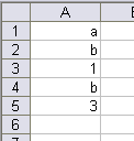
The problem – to create an array containing only the unique items from an expanding column list. In other words, if items are typed down column A, what is the formula that will return the unique items? The following example further illustrates the problem.

In this case, the array should be {“a”;”b”;1;3}. Then, if additional values
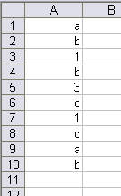
are added:

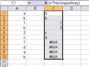
the array should be {“a”;”b”;1;3;”c”;”d”}. The answer to this problem has eluded me for years, but with recent input from Bob and Laurent, I have successfully constructed a solution to this problem. The formula is somewhat long, so it is necessary to define parts of the formula to simplify the final form.
Create a defined name with a Name of TheList and a Refers to of:
This formula creates the expanding range for the items as they are entered
into column A.
Define sArray as:
ROW(INDIRECT(“1:”&SUM(N(MATCH(TheList,TheList,0)=ROW(TheList))))))-1
This formula contains several important elements that require explanation. The formula
returns an array of positions for the unique items that is the same size as the TheList array, where the duplicates items are now represented by empty strings. The formula
returns an array of numbers from 1 to n, where n is the number of unique items in the list, as calculated by the formula
.
What is desired is an array that contains the unique positions with no empty strings. This is accomplished by the use of the SMALL function which, along with the LARGE function, is unique among Excel functions in its ability to create different sized arrays than the array used in the 1st argument if the 2nd argument is also an array. The -1 is used to adjust the item positions for use in the formula shown below.
Define TheUniqueArray as:
The formula
is an array of single element arrays, as explained in detail in the 1st issue of EEE. It can be converted into a normal array by using the N or T functions. Both N and T are used here since TheList can contain either text or numeric items.
WARNING: This formula can take a while to calculate if TheList is long. One thousand items took a couple of seconds on my Latitude D810.

Most of what I learned about “power” formulas came from studying the EEE articles written by these 3 gurus, along with many of their old newsgroup postings.
When I googled by own postings for unique value formulas, I found this array formula from 2004:
=INDEX($A$1:$A$10,SMALL(IF(ROW($A$1:$A$10)=MATCH($A$1:$A$10,$A$1:$A$10,0),ROW($A$1:$A$10)),ROW()))
The formula has a David Hager “feel” to it or may have even been borrowed from another formula guru, Peo Sjoblom.
Jason
Ouch, my head hurts! Nice work.
I have used the following in the past:
{=SUM(COUNTIF(INDIRECT(“‘Sheet1’!B2:B”&COUNTA(‘Sheet1’!B:B)),INDIRECT(“‘Sheet1’!B2:B”&COUNTA(‘Sheet1’!B:B)))/(COUNTIF(INDIRECT(“‘Sheet1’!B2:B”&COUNTA(‘Sheet1’!B:B)),INDIRECT(“‘Sheet1’!B2:B”&COUNTA(‘Sheet1’!B:B)))^2))}
This counts all of the unique entries in column B of Sheet1 – B2 is used as the start cell to account for the header / field name. COUNTA() is used to find the number of non-blank cells and is then converted from a text string using c.
Although this is not as tidy or compact as your method, it does seem to work quite well – calculation of just over 1000 records takes less than a second on my Latitude D600.
The INDIRECT() part can be removed to work with a static range as follows (also posted as a comment under yesterday’s post):
{=SUM(COUNTIF(RANGE,RANGE)/(COUNTIF(RANGE,RANGE)^2))}
One other possibility is to make use of Excel’s FREQUENCY function. This function calculates how often values occur with a range of values and returns an array of these values.
When the values being checked and the range of values are the same, Excel creates an array of unique values and FALSE for every value that exists more than once in the list since it is not possible to have values that occur between two of the same value.
For instance using the array formula: =IF(FREQUENCY(TheList,TheList)>0,TheList)
with TheList: 1,3,2,2,4,5,1,1
yields:
1
3
2
FALSE
4
5
FALSE
FALSE
FALSE
If this is combined with a function to bring back the smallest n values in the array (created with the frequency function), the array of unique values from the original list can be created.
He is my array formula:
=SMALL(IF(FREQUENCY(TheList,TheList)>0,TheList),ROW(INDIRECT(“1:”&COUNT(IF(FREQUENCY(TheList,TheList)>0,1)))))
I am curious how this does from a calculation perspective compared to some of the other suggestions. Maybe when I have some free time…
Dan
Forgot to mention it, but this solution only works with numerical data…
Dan
How about checking the newsgroups. This has been answered several times over the years.
Anyway, lots of OFFSET calls (or other volatile function calls) always kills performance.
If the result would be used as a term in longer formulas, there may be better alternative formulas that don’t require such an array. If the result would populate another range, there’s a much better alternative that doesn’t call any volatile functions.
Define TheList as
=$A$1:INDEX($A:$A,COUNTA($A:$A))
Topmost cell (make it C1)
=INDEX(TheList,1)
Next cell (C2)
=INDEX(TheList,MATCH(0,COUNTIF(C$1:C1,TheList),0))
The last is an array formula. Fill the last formula down as far as needed. The filled formulas may also take a long time to calculate the first time, but they won’t recalculate every time anything triggers recalculation.
There are newsgroup postings with this technique at least as far back as 2000. There were likely even older postings, but Google doesn’t seem to do well with the Deja News archive they bought.
Nice to know the blogger finally reinvented this wheel.
Where did you think I got my posting ideas?
I am having a surprising amount of trouble trying to adjust this method to account for a header row… Could someone please explain how they would go about it?
Why not just use a pivot table to determine the unique values and the count of each unique value? It’s simple and quick, and it will also update as you add more data to the original listing – all you have to do is refresh the results.
Pivot tables don’t update automatically. Refresh is nice, but it’s manual. Pivot tables also require field labels in the top row, they span at least 2 columns, and you can’t always ensure the original order is reproduced.
What am I doing wrong, because these don’t work:
because (“‘Sheet1’!B2:B”or this because “1:”
=SMALL(IF(MATCH(TheList,TheList,0)=ROW(TheList),ROW(TheList),””),
ROW(INDIRECT(“1:”&SUM(N(MATCH(TheList,TheList,0)=ROW(TheList))))))-1
Thanks
Vera
If you’ve copied the formulas directly from the web page you’ll need to change the quotes in “1:” because they’re a different character and they don’t work in the Excel formula. I think all the other quotes are correct.
Also, if you’ve defined your list as starting from a row other than row one (you’ve mentioned B2) then you’re going to need some adjustments to the other formulas.
Good work.
But how could this technique used to populate a combobox with TheUniqueArray
Regards
@Eugene: Try this: Replace all calls to ROW(Table1[Name]) with ROW(Table1[Name])-SMALL(ROW(Table1[Name]),1)+1
@Belarbi: Trying to get data validation working to. What is the reason for this failing when trying to use data validation?