Months of the World

While putting together the last post, something caught my eye. Something that I’d never noticed about cell formatting.

It was a custom cell format that was created without my action: [$-1409]dddd, d mmmm yyyy
It looked like a date format, but what was that [$-1409] ?!
Recognising 1409 as the New Zealand locale ID, I guessed it had something to do with Regional Settings.

You can actually change your date format for any recognised Country.
Time to play! Fancy your dates in Dutch?

Click your date cell.
From the Format menu, select Cells.
From the Number tab, select Date.
Choose the Locale (location) from the drop down box.

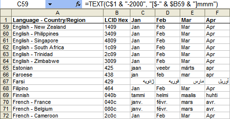
I wanted to see them all at once, so I copied a List of Locale ID (LCID) Values as Assigned by Microsoft, pasted them into Excel and wrote a formula for displaying all of the translations:

3D User Defined Functions

By Myrna Larson and David Hager

Presented below are 3 UDF’s (SumProduct3D, SumIf3D, CountIf3D) that
provide a useful method of returning a variety of information from 3D
ranges. Each of these functions use a 3D range argument (written as per
the usual Excel protocol) as a string. This string is processed by the
Parse3DRange function, which returns sheet positions and the range argument
in variables that are used by these functions.

Function SumProduct3D(Range3D As String, Range_B As Range) _
    As Variant
 
    Dim sRangeA As String
    Dim sRangeB As String
    Dim Sheet1 As Integer
    Dim Sheet2 As Integer
    Dim Sum As Double
    Dim n As Integer
 
    Application.Volatile
 
    If Parse3DRange(Application.Caller.Parent.Parent.Name, _
      Range3D, Sheet1, Sheet2, sRangeA) = False Then
      SumProduct3D = CVErr(xlErrRef)
      Exit Function
    End If
    sRangeB = Range_B.Address
 
    Sum = 0
    For n = Sheet1 To Sheet2
      With Worksheets(n)
        Sum = Sum + Application.WorksheetFunction.SumProduct( _
    .Range(sRangeA), .Range(sRangeB))
      End With
    Next
    SumProduct3D = Sum
  End Function
 
Function SumIf3D(Range3D As String, Criteria As String, _
    Optional Sum_Range As Variant) As Variant
 
    Dim sTestRange As String
    Dim sSumRange As String
    Dim Sheet1 As Integer
    Dim Sheet2 As Integer
    Dim n As Integer
    Dim Sum As Double
 
    Application.Volatile
 
    If Parse3DRange(Application.Caller.Parent.Parent.Name, _
      Range3D, Sheet1, Sheet2, sTestRange) = False Then
      SumIf3D = CVErr(xlErrRef)
    End If
 
    If IsMissing(Sum_Range) Then
      sSumRange = sTestRange
    Else
      sSumRange = Sum_Range.Address
    End If
 
    Sum = 0
    For n = Sheet1 To Sheet2
      With Worksheets(n)
        Sum = Sum + Application.WorksheetFunction.SumIf(.Range _
    (sTestRange), Criteria, .Range(sSumRange))
      End With
    Next n
    SumIf3D = Sum
  End Function
 
Function CountIf3D(Range3D As String, Criteria As String) _
    As Variant
 
    Dim Sheet1 As Integer
    Dim Sheet2 As Integer
    Dim sTestRange As String
    Dim n As Integer
    Dim Count As Long
 
    Application.Volatile
 
    If Parse3DRange(Application.Caller.Parent.Parent.Name, _
      Range3D, Sheet1, Sheet2, sTestRange) = False Then
      CountIf3D = CVErr(xlErrRef)
      Exit Function
    End If
 
    Count = 0
    For n = Sheet1 To Sheet2
        With Worksheets(n)
          Count = Count + Application.WorksheetFunction.CountIf( _
      .Range(sTestRange), Criteria)
        End With
    Next n
    CountIf3D = Count
  End Function
 
Function Parse3DRange(sBook As String, SheetsAndRange _
    As String, FirstSheet As Integer, LastSheet As Integer, _
    sRange As String) As Boolean
 
    Dim sTemp As String
    Dim i As Integer
    Dim Sheet1 As String
    Dim Sheet2 As String
 
    Parse3DRange = False
    On Error GoTo Parse3DRangeError
 
    sTemp = SheetsAndRange
    i = InStr(sTemp, “!”)
    If i = 0 Then Exit Function
 
    ‘next line will generate an error if range is invalid
   ‘if it’s OK, it will be converted to absolute form
   sRange = Range(Mid$(sTemp, i + 1)).Address
 
    sTemp = Left$(sTemp, i – 1)
    i = InStr(sTemp, “:”)
    Sheet2 = Trim(Mid$(sTemp, i + 1))
    If i > 0 Then
      Sheet1 = Trim(Left$(sTemp, i – 1))
    Else
      Sheet1 = Sheet2
    End If
 
    ‘next lines will generate errors if sheet names are invalid
   With Workbooks(sBook)
    FirstSheet = .Worksheets(Sheet1).Index
    LastSheet = .Worksheets(Sheet2).Index
 
    ‘swap if out of order
   If FirstSheet > LastSheet Then
      i = FirstSheet
      FirstSheet = LastSheet
      LastSheet = i
    End If
 
    i = .Worksheets.Count
    If FirstSheet >= 1 And LastSheet < = i Then
      Parse3DRange = True
    End If
    End With
Parse3DRangeError:
    On Error GoTo 0
    Exit Function
 
End Function  ‘Parse3DRange

Editor’s Note: I didn’t like that the second argument was a range that had to mirror the 3D-ness of the first string-range. I change the parsing function to return an array of ranges so that you could put any two equally sized ranges in as arguments and one, both, or neither have to be 3D. The downside is that both arguments have to be strings.

Function SumProduct3D2(sRng1 As String, sRng2 As String) _
    As Variant
 
    Dim vaRng1 As Variant, vaRng2 As Variant
    Dim rTemp As Range
    Dim i As Long
    Dim Sum As Double
    Dim rCell As Range
   
    Application.Volatile
   
    vaRng1 = Parse3DRange2(Application.Caller.Parent.Parent, sRng1)
    vaRng2 = Parse3DRange2(Application.Caller.Parent.Parent, sRng2)
   
    For i = LBound(vaRng1) To UBound(vaRng1)
        Sum = Sum + (vaRng1(i).Value * vaRng2(i).Value)
    Next i
   
    SumProduct3D2 = Sum
   
  End Function
 
Function SumIf3D2(Range3D As String, Criteria As String, _
    Optional Sum_Range As String) As Variant
 
    Dim Sum As Double
    Dim vaRng1 As Variant, vaRng2 As Variant
    Dim i As Long
   
    Application.Volatile
   
    If Len(Sum_Range) = 0 Then
      Sum_Range = Range3D
    End If
 
    vaRng1 = Parse3DRange2(Application.Caller.Parent.Parent, Range3D)
    vaRng2 = Parse3DRange2(Application.Caller.Parent.Parent, Sum_Range)
   
    Sum = 0
    For i = LBound(vaRng1) To UBound(vaRng1)
        Sum = Sum + Application.WorksheetFunction.SumIf(vaRng1(i), Criteria, vaRng2(i))
    Next i
   
    SumIf3D2 = Sum
   
End Function
 
Function CountIf3D2(Range3D As String, Criteria As String) _
    As Variant
 
    Dim i As Long
    Dim Count As Long
    Dim vaRng1 As Variant
   
    Application.Volatile
 
    vaRng1 = Parse3DRange2(Application.Caller.Parent.Parent, Range3D)
 
    Count = 0
    For i = LBound(vaRng1) To UBound(vaRng1)
        Count = Count + Application.WorksheetFunction.CountIf(vaRng1(i), Criteria)
    Next i
   
    CountIf3D2 = Count
   
End Function
 
Function Parse3DRange2(wb As Workbook, _
                        SheetsAndRange As String) As Variant
 
    Dim sTemp As String
    Dim i As Long, j As Long
    Dim Sheet1 As String, Sheet2 As String
    Dim aRange() As Range
    Dim sRange As String
    Dim lFirstSht As Long, lLastSht As Long
    Dim rCell As Range
    Dim rTemp As Range
   
    On Error GoTo Parse3DRangeError
 
    sTemp = SheetsAndRange
       
    ‘if it’s 3d, rtemp will be nothing
   On Error Resume Next
        Set rTemp = Range(sTemp)
    On Error GoTo Parse3DRangeError
   
    ‘if it’s 3d, parse it
   If rTemp Is Nothing Then
       i = InStr(sTemp, “!”)
       If i = 0 Then Err.Raise 9999
   
       ‘next line will generate an error if range is invalid
      ‘if it’s OK, it will be converted to absolute form
      sRange = Range(Mid$(sTemp, i + 1)).Address
   
       sTemp = Left$(sTemp, i – 1)
       i = InStr(sTemp, “:”)
       Sheet2 = Trim(Mid$(sTemp, i + 1))
       If i > 0 Then
           Sheet1 = Trim(Left$(sTemp, i – 1))
       Else
           Sheet1 = Sheet2
       End If
   
       ‘next lines will generate errors if sheet names are invalid
      With wb
           lFirstSht = .Worksheets(Sheet1).Index
           lLastSht = .Worksheets(Sheet2).Index
       
           ‘swap if out of order
          If lFirstSht > lLastSht Then
               i = lFirstSht
               lFirstSht = lLastSht
               lLastSht = i
           End If
             
           ‘load each cell into an array
          j = 0
           For i = lFirstSht To lLastSht
               For Each rCell In .Sheets(i).Range(sRange)
                   ReDim Preserve aRange(0 To j)
                   Set aRange(j) = rCell
                   j = j + 1
               Next rCell
           Next i
       End With
       
       Parse3DRange2 = aRange
    Else
        ‘range isn’t 3d, so just load each cell into array
       For Each rCell In rTemp.Cells
            ReDim Preserve aRange(0 To j)
            Set aRange(j) = rCell
            j = j + 1
        Next rCell
       
        Parse3DRange2 = aRange
    End If
   
Parse3DRangeError:
    On Error GoTo 0
    Exit Function
 
End Function  ‘Parse3DRange
Date Separator and Regional Settings

I’m a New Zealander and that’s what I’ll be writing on 7 March for NZ’s Census 2006.
There has been a bit of news in this country about that issue. Until now, you could not record your ethnicity as “New Zealander” in New Zealand! Strange but true. But that’s all about to change.

<shakes head> Back to Excel… where was I?

If you live in a non-US country, you might have been caught by some applications using mm/dd as the default date format.
It has often led to problems for me.
Take the date: 7th of March. It could be written 07/03 (as we do in New Zealand) or 03/07 as it is in the US.

It’s really quite annoying that the first 12 days of the month could be mistaken for dd/mm or mm/dd.
There’s no use crying about it… I just find a way to deal with it.

The way I go is to always format the month as text. In other words dd-mmm-yyyy which appears as 07-Mar-2006
I have done it this way for a long time.
Over the years I’ve noticed an unfortunate problem surfacing. Some computers format my date cells differently!
Instead of the format 07-Mar-2006, it comes out as 07/Mar/2006. Those slashes look out of place and really ugly!

It turns out to be an Excel vs. Regional Settings quirk.

Scenario 1:

    You format a cell using the same date separator as that specified in Regional Settings. The date separator will, from then on, always inherit from Regional Settings.

    Excel stores the date separator as a forward slash.
    eg. Regional Settings = dd-MMM-yyyy then I format a cell as dd-mmm-yyyy. Excel stores the format as dd/mmm/yyyy.

Scenario 2:

    You format a cell using a different date separator to that specified in Regional Settings. The cell will then never inherit from Regional Settings.
    Internally Excel will prefix the date separator with a hidden backslash. ActiveCell.NumberFormat will not show the hidden blackslash.

Since my computer’s Regional Settings has a hyphen (-) for a date separator, I activated the “inherit” mode for the date separator.

The general rule is, when you want to enforce date separators, prefix them with a backslash.
In my case, I just need to change my cell formats to: dd-mmm-yyyy

Some Dynamics on www.jkp-ads.com

Hi everyone,

Here’s a newby showing off his newly acquired tricks with asp and VBScript.

(I know, old stuff, badly written code an it looks horrid, but hey, it works!)

I’ve added a database to my site and am slowly putting some interactivity in place.

First step I took was to give you the opportunity to rate my articles.
The following pages have a set of 10 stars at their bottom (how’s that for bad language :-) ) which you can click to rate the article (1 is terrible, 10 is excellent):


www.jkp-ads.com/articles/ControlHandler04.asp


www.jkp-ads.com/articles/CorruptFiles.asp


www.jkp-ads.com/articles/DistributeMacro11.asp


www.jkp-ads.com/articles/ExcelNames11.asp


www.jkp-ads.com/articles/StartupProblems.asp


www.jkp-ads.com/articles/WebQuery.asp

Have fun!

Regards,

Jan Karel Pieterse
JKP Application Development Services

Sorting Arrays of User Defined Types

I have an array of user defined types. The type has three elements and I need to sort on all three. Surprisingly, I’ve never had to sort an array of udt’s before. Here’s how I did it:

Type MyInfo
    lType As Long
    sName As String
    dStart As Date
End Type
 
Sub Start()
   
    Dim aInfo(0 To 4) As MyInfo
    Dim i As Long
    Dim vaTypes As Variant
    Dim vaNames As Variant
    Dim vaDates As Variant
   
    ‘fill the array with some unsorted data
   vaTypes = Array(2, 1, 1, 2, 1)
    vaNames = Array(“Joe”, “Bob”, “Bob”, “Joe”, “Joe”)
    vaDates = Array(#1/1/2006#, #2/1/2006#, #1/15/2006#, #6/30/2005#, #1/8/2006#)
   
    For i = 0 To 4
        aInfo(i).lType = vaTypes(i)
        aInfo(i).sName = vaNames(i)
        aInfo(i).dStart = vaDates(i)
    Next i
   
    ‘call the sort procedure
   SortInfo aInfo
   
    ‘output the results to the immediate window
   For i = LBound(aInfo) To UBound(aInfo)
        Debug.Print aInfo(i).lType, aInfo(i).sName, aInfo(i).dStart
    Next i
   
End Sub
 
Sub SortInfo(ByRef aInfo() As MyInfo)
   
    Dim i As Long, j As Long
    Dim tTemp As MyInfo
   
    ‘standard bubble sort loops
   For i = LBound(aInfo) To UBound(aInfo) – 1
        For j = i To UBound(aInfo)
            ‘sort on the first element
           If aInfo(i).lType > aInfo(j).lType Then
           
                SwapInfo aInfo, i, j
           
            ‘if the first element is the same, sort on the second
           ElseIf aInfo(i).lType = aInfo(j).lType And _
                aInfo(i).sName > aInfo(j).sName Then
               
                SwapInfo aInfo, i, j
           
            ‘if the first two elements are the same, sort on the third
           ElseIf aInfo(i).lType = aInfo(j).lType And _
                aInfo(i).sName = aInfo(j).sName And _
                aInfo(i).dStart > aInfo(j).dStart Then
               
                SwapInfo aInfo, i, j
               
            End If
        Next j
    Next i
   
End Sub
 
Sub SwapInfo(ByRef aInfo() As MyInfo, ByVal lOne As Long, ByVal lTwo As Long)
 
    Dim tTemp As MyInfo
   
    tTemp = aInfo(lOne)
    aInfo(lOne) = aInfo(lTwo)
    aInfo(lTwo) = tTemp
   
End Sub

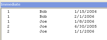
immediate window showing sorted output

Is there an easier way?

Bible Workbook

File this under “The last thing you’d expect from John Walkenbach.” It’s the Bible in an Excel workbook.

I found a text file with the complete King James Version of the Bible. I wrote a few macros and dumped it all into an Excel workbook. Each book is on a separate worksheet, and each verse is in a separate cell.

It has a handy hyperlink table of contents so you can jump to any book. I also wrote some summary formulas to calculate the number of characters in each book, and the average number of characters per verse. Then I added a word count feature: Enter a word and it displays the number of occurrences in each book. Finally, I set up a User Form that displays a random verse.

You can download it here. It’s a 1.8 Mb zip file, and it expands to a 6.1Mb Excel workbook. Even if you have no interest in the content, you may discover a few useful techniques. You’ll need to enable macros to use the random verse feature.

3D Array Formulas

Created by Laurent Longre

The problem – to make a 3D worksheet array formula. What this means is to
create an array representing a z-range (a range across worksheets) that
evaluates in the formula bar as an array. The 3D range used in Excel, i.e.

Sheet1:Sheet4!A2:B5

does not behave that way. I suspect that nearly everyone on the EEE list
has tried to do this and found that it was not possible. However, Laurent
found that it was possible, given some advanced formula tricks. The INDIRECT
function can return a 3D reference if it is operated on by the N function.
An illustration of this type of formula is shown below.

3D Diagonal Formula –

=SUM(N(INDIRECT(“Sheet”&{1,2,3}&”!”&ADDRESS({1,2,3},{1,2,3}))))

returns the sum of Sheet1!A1, Sheet2!B2 and Sheet3!C3. How does it work?

“Sheet”&{1,2,3}&”!”&ADDRESS({1,2,3},{1,2,3}) evaluates to the array of
strings.

{“Sheet1!$A$1?,”Sheet2!$B$2?,”Sheet3!$C$3?}

When the INDIRECT function operates on this array, the expected array of
values appear (by highlighting in the formula bar and pressing F9), but
for some reason this array cannot be used by Excel functions. The use of
the N function creates an array that can be used, so that the SUM function
returns the desired result.