Created by Laurent Longre:
The problem – how to create an array of filtered items in a column
list. The SUBTOTAL function allows you to operate on an array of this
type with a limited number of worksheet functions, but it does not
expose the array for formula manipulation. Laurent came up with an
elegant solution to this problem, based on an obscure behavior of
the OFFSET function. It turns out that when an array is used as the
2nd argument of OFFSET, such as
=OFFSET(Rge,ROW(Rge)-MIN(ROW(Rge)),,1)
an array of RANGES is returned. If the array is properly sized, as in
this example, the OFFSET function returns a separate single cell range
for each cell in the original range(Rge). Thus, if this array of arrays
is operated on by the SUBTOTAL function, each single cell range gets
evaluated separately. So, the formula
=SUBTOTAL(3,OFFSET(Rge,ROW(Rge)-MIN(ROW(Rge)),,1))
evaluates as 1 for each cell that is visible and as 0 if the cell is not
visible. The use of 3 as the 1st argument in SUBTOTAL counts the number of
items in the visible range. Since there is only one item in each range,
the answer can only be 0 or 1. Thus, this formula can be used as an array
which indicates the rows in the list that are filtered and unfiltered. If
you want to returns an array of items in the column list, then use:
=IF(SUBTOTAL(3,OFFSET(Rge,ROW(Rge)-MIN(ROW(Rge)),,1)),Rge,””)
Editor’s example:
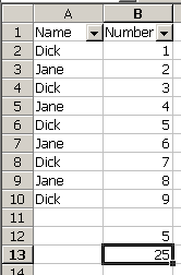
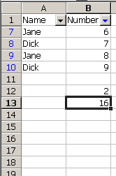
The range on the left is unfiltered. The range on the right is filtered on the Number column for Top 4.

|

|
The formulas are:
B12: =SUM((Rge1="Dick")*(SUBTOTAL(3,OFFSET(Rge2,ROW(Rge2)-MIN(ROW(Rge2)),,1))))
B13: =SUM((Rge1="Dick")*(SUBTOTAL(9,OFFSET(Rge2,ROW(Rge2)-MIN(ROW(Rge2)),,1))))
The OFFSET function used with SUBTOTAL returns an array which can be used as one element of an array formula. SUBTOTAL without OFFSET returns only a scalar value, not an array. These formulas not only limit based on “Dick” being in the name column, but also on the row being unfiltered.
Hi,
I tried this and it works great. However, if a row is hidden (Format – Row – Hide) as opposed to filtered out, then the formula does not work.
I have previously tried to get around that by using the CELL function, which *does* work on the more generic ‘hidden’ property, but it appears that there is another issue.
Excel does not seem to recognise the hiding (and unhiding) of columns (and rows) as an ‘event’ which triggers recalculation.
I even added in a volatile element to the formuale – mutiplying by (NOW()/NOW()) – but that still requires the users to press F9 to actually force a re-calc.
I have previously posted on this in the ms public newsgroups (http://tinyurl.com/cygvc) and (http://tinyurl.com/dgxet) the first is the moe recent and got a response, but I was hoping someone here may have a better suggestion?
Thanks,
Alan.
microsoft.public.excel.worksheet.functions
Sunday, April 17, 2005 11:38 AM
A fellow named Domenic responded to a question I had for this same thing. We exchanged several emails – thanks Domenic!
Two things I wanted to know: first how to use other measures of central tendency beyond sum, count, average, stdev, etc. to measure a list of sales ratios. The following array formula was used for median, avedev, geomean, harmean:
{=MEDIAN(IF(SUBTOTAL(3,OFFSET($AF$2:$AF$64,ROW($AF$2:$AF$64)-MIN(ROW($AF$2:$AF$64)),0,1)),$AF$2:$AF$64))}
and works fine.
Also wanted to do a calculation on the same list but for only those visible rows that were compared to a list of parameters. EG list of Quarters (1 – 4) and the central tendency of any visible rows that were in a particular quarter
Give from visible rows
Term Median GeoMean Mean …
1
2
3
4
{=MEDIAN(IF((SUBTOTAL(3,OFFSET($E$2:$E$64,ROW($E$2:$E$64)-MIN(ROW($E$2:$E$64)),0,1)))*($E$2:$E$64=$E67),$AF$2:$AF$64))}
I think the use of Row(…) solves your problem
HTH
doco
I meant to say “should” – it works for me with all hidden and or filtered rows. The only real problem I have had with it is pasting results to another sheet: you will not want to use PasteSpecial PasteAll as it will give reference to the entire referenced column UsedRange; which creates some unforseen problems later on.
Dick: is there a way to edit posts? :-(
ross’s ducks…urrrrrrrggggggggg, complex formulas!!!!
Hi doco,
Thanks for your response.
I must be dim, but I cannot see how that would work?
oesn’t that still require the user to manually re-calculate (regardless of whether they have calculation mode set to automatic or not)?
Thanks for your assistance,
Alan.
Hello,
This solution looks fanastic, but I can’t get it to work.
My initial motivations were to apply it to an AVEDEV function across a range, but after my implementation failed, I set about testing the example formula with exactly the same data as shown in your example. I replicated exactly your example and copied the code (right down to the values and named ranges).
The result of applying the sample equation is “#VALUE!” (in both cases).
Using the Evaluate Formula function, I notice that it seems to be failing on the filtering function “Rge1=”Dick””. Where “Rge1? should be shown it displays “#VALUE1? – but everything else seems to resolve properly.
Suspecting that I needed some add-ins, I enabled “Analysis Toolpak” through “Solver Addin” – this has not improved things.
This is an excellent website – if I can get a reply to this, you will make my day!
Regards,
Justin
Justin: Make sure you have named ranges Rge1 and Rge2 or use actaul range references in your place. Make sure you’re entering those array formulas with Control+Shift+Enter, not just Enter. See
http://www.dicks-blog.com/archives/2004/04/05/anatomy-of-an-array-formula/
To doco (who suggested how to use GEOMEAN and filtering together)
I used you suggestion but couldn’t get it to work when some data cells in my array were blank… therefore I went back to basics
If anyone is looking to find the geological mean and filter data at the same time this is how I did it:
=SUBTOTAL(6,I4:I37)^(1/(SUBTOTAL(2,I4:I37)))
where I4:I37 is my range
SUBTOTAL (6) gives the product of the cells in the range that are unfiltered
SUBTOTAL (2) counts the number of cells
I know this isn’t about using offset but I thought it applied to some of the suggestions on this (excellent) page
With regards,
Carl
So the geological mean of Cretaceous and Triassic is Jurassic then? ;-)
Nice formula for a filtered Geomean btw.
Suppose I have two columner arrays A and B and want to calculate the sum of the products of A and B under various autofilter conditions in a single cell. Can this be done using Subtotal function? In the absence of an elegant shortcut, I am forced to create another array C and the use the Subtotal function on it.
Thanks,
Gary
I think I may have solved my own question by trying:
=SUM(SUBTOTAL(9,OFFSET(Range A,ROW(Range A)-MIN(ROW(Range A)),,1))*SUBTOTAL(9,OFFSET(Range B,ROW(Range B)-MIN(ROW(Range B)),,1)))
This seems to be equivalent to
=Subtotal(9, Range C) where Range C = (Range A) X (Range B)
This enables me to eliminate the creation of the large intermediate array C which was only created so that it could be summed with autofilters.
Please confirm or comment if anyone knows of situations where this would not be true.
Gary