39 thoughts on “INDIRECT and Dynamic Ranges”

1. You should make your function Volatile as well Dick, at least to be consistent with INDIRECT().

2. option #3:

   Instead of using
   =MAX(INDIRECT(List2)),
   Charlie must use:

   =MAX(List2)

3. INDIRECT does not evaluate formulas that use worksheet functions, and if the defined name represents a formula and not a simple reference, it’ll error out. A possible Option #3 is to use XLM’s EVALUATE.

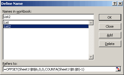
   Define the name “List2? as:

   =MAX(OFFSET(…))

   Define another name “Eval” as:

   =EVALUATE(List2)

   Call as:

   =Eval

   Regards,
   Jason

4. Doh! EVALUATE is overkill in this case. Just use:

   =List2

   Jason

5. Daniel: The point is that “List2? is created via a formula and can’t be hardcoded. Therefore, the indirect is necessary, although I left all that background out of the post.

   Jason: I couldn’t get that to work. Even if it did, you would need List2 to return a scalar value and not a range reference. That would be fine if you only wanted to take the MAX of the range, but if you hand more formulas that used that range, you would need one name for every formula. Am I right on that, or am I missing something?

6. Thank you everyone for your help. Juan Pablo is correct. Whatever UDF is created it needs to be volatile. That is tha majic of the INDIRECT function.

   I created a validated dropdown box with 4 items to choose from. Each items is a named range consisting of one column from a large Excel database. When the user selects the item the INDIRECT function reads the selection and finds the correct named range. There are multiple calculations being done; MAX, MIN, SUM, AVERAGE, etc. all calculating the selected item from the dropdown. The INDIRECT function is being used in all calculations.

   I use one poor work around. The range begins at row 1 and ends at row 65536. The problem with this is wasted process time. My computer has to look through all those cells for nothing.

7. Thanks Dick, I didn’t get the point about creating List2 dynamicaly (perhaps because I disagree about this specific usage). :-)

   Charlie,

   I disagree with the way you are adressing (!) the problem.

   In my view, the select you make in the dropdown should trigger another change value (let’s call it Shift).
   Even with very complex spreadsheet, the Shift can be obtained via a VLOOKUP() to an array that would determine the proper offset depending on the dropdown value.

   Then your List2 name would use the Shift name (in the OFFSET function) to correctly define the proper range.

   This method is perfectly scalable to any amount of ranges (doesn’t need to define one Name for each choice).

   And the spreadsheet dependencies are straightforward. No call to volatile.

   My two cents anyway (but it’s your call after all). :-)

   Daniel

8. Dick said:

   One way to get around the problem is to just reproduce the dynamic range name formula in the cell.

   =MAX(OFFSET(Sheet1!$B$6,0,0,COUNTA(Sheet1!$B:$B)-1))

   That works, but now when you change List2, you have to remember to change this formula too, not to mention all the other formulas that use this.

   The last part is not necessarily correct (about needing to change the formula when list2 changes).

   As identified, indirect unfortuantely does not work with dynamic ranges, but if you have named references to a specific cell and the size of the relevant range can be determined by means of other associated data you can use indirect If you have no associated data, and cannot determine what the maximum size of that list will be, you’re out of luck.

   For example, here’s a formula from one of my projects, that is then wrapped in sum, max, median, average, or “=value” statements (- and all return the correct values)

   OFFSET(INDIRECT(“tournamentsCellStart_” & $A$3),RankingYearStart,0,countTournaments_Selected,1)

   and the absolute reference $A$3 is determined by some means, and resolves to:

   tournamentsCellStart_Chris =Tournaments!$G$3
   tournamentsCellStart_Colin=Tournaments!$I$3
   etc

   countTournaments_Selected is determined by a set of date range conditions in named formulas.

   But indirect here operates only on the (conditionally selected) starting cell for the offset function, so no problems
   n

9. Question: Will using DINDIRECT() work, if I’m trying to use this to provide a dynamic range for data validation?

   In my attempts, INDIRECT(dynamic range) doesn’t work for LIST data validation.

   I also tried using DINDIRECT(dynamic range), as the argument for LIST data validation (and implementing the above code). Excel then returns the message “A named range you specified cannot be found”.

   As background: The dynamic range is already defined, and can be successfully accessed via INDEX/MATCH and so on.

10. Hi the DINDIRECT function seems like a great solution to me but when i try to make it volatile (just by inserting application.volatile as the first line) it breaks and I get a #VALUE! error in my cell. If anyone has any advice on how to fix this i’d really appreciate it.
    Thanks,

    Ben

11. Hello,

    the question is, why do you actually need INDIRECT().

    Usually you want to use INDIRECT() in data validation, where the validation list depends on the choice in another cell.

    I have certain success with the following:

    1) Let List1 and List2 be your dynamic ranges.

    2) Let List be defined as {“List1?,”List2?}

    3) Let A1 be validated as List

    4) Let your validation range be validated as list like this:

    =CHOOSE(MATCH($A$1,Lists,0),List1,List2)

    I know this doesn’t answer the question, but it serves as a workaround for one specific case. The INDIRECT() is to be avoided with calculated ranges (that do not appear in the name box). Everybody knows that INDIRECT() is to be avoided with closed workbooks and yep, this is another limitation.

    Martin

12. Oh, sorry for the typo, of course it should read:

    =CHOOSE(MATCH($B$7;List;0);List1;List2)

13. In addition to Martin Krals statement on the combination of Choose and Match, I want to mention the following. For the dynamic selection to work flawless, it is necessary to have the same sequence in the CHOOSE list as you have defined in the dynamic range list. If you don’t use the same sequence then the wrong dynamic range will be set.

14. Hi Dick,

    I have used the code you gave on 01.03.2005 for the following purpose.
    In cell A1 of a sheet I have a validation list containing name of 3 sheets HDFC, SBOP, SBIL. I have named ranges

    Recobank=”‘”&Reco!$A$2&”‘!”
    RecoAmt=Dindirect(“‘”&RecoBank&”‘!i4?)

    Now the RecoAmt should result in Value contained in Cell I4 of sheet named HDFC. But it is not giving me any results. What should be the reasons ?

    Regards
    CA kanwaljit singh Dhunna

15. Hi,
    Just to mention that in the above case
    RecoAmt=Evaluate(“‘”&RecoBank&”‘!i4?) is working fine.

16. Hi Dick,

    I found this post while searching for a work around to Indirect referencing a dynamic range name limitation.

    I am using a scroll bar to scroll through tables based on Week/month.
    I have a cell that stores the scroll bar value (C9).
    I then use in another cell (C22) a string formula”Dashboard_Data_Table”&$C$9.
    I am then using the following to dynamically update the data =INDEX(INDIRECT(C22),Rownum,ColNum).

    The problem I was having was the Indirect Dynamic ref failure. I searched google and bang! DIndirect has resolved the problem. Thank you so much. I now have a dynamic dashboard that can scroll through different time scaled tables. This allows users to stay on one screen a push 12 months worth of data through the various dashboard charts. I am sure I would have found another work around eventually however, this was quick, simple and worked a charm.

    Thanks again

    devoted ddoe reader

    Tim B

17. Hi Dick,

    I found this post while searching for a work around to Indirect referencing a dynamic range name limitation.

    I am using a scroll bar to scroll through tables based on Week/month.
    I have a cell that stores the scroll bar value (C9).
    I then use in another cell (C22) a string formula”Dashboard_Data_Table”&$C$9.
    I am then using the following to dynamically update the data =INDEX(INDIRECT(C22),Rownum,ColNum).

    The problem I was having was the Indirect Dynamic ref failure. I searched google and bang! DIndirect has resolved the problem. Thank you so much. I now have a dynamic dashboard that can scroll through different time scaled tables. This allows users to stay on one screen a push 12 months worth of data through the various dashboard charts. I am sure I would have found another work around eventually however, this was quick, simple and worked a charm.

    Thanks again

    devoted ddoe reader

    Tim B

18. Ran into this problem today. Had no idea about the problem of dynamic ranges and indirect references. Ugh.

    So, I also took a UDF approach, but decided on a simple string return:

    Public Function DRNG_ADDRESS(range_name As String) As String
    ‘   Takes the name of a dynamic range and returns
    ‘   the address of that name.

        Application.Volatile
        Dim rng As Range
           
        ‘ Set the range variable.
        Set rng = Range(range_name)
       
        ‘ Return the range variable address. Also include the
        ‘ sheet name so that it will work across separate worksheets.
        DRNG_ADDRESS = rng.Parent.Name & “!” & rng.Address
       
    End Function

    So, using a VLOOKUP to get the dynamic range name (which I have in ANOTHER dynamic range–don’t ask!), I can pull the name, return the DR address as a string (along with the sheet name), and use the indirect in the DV.

    The formula’s pretty easy, even with the lookup:

    =DRNG_ADDRESS(VLOOKUP(D6,drRanges,2,FALSE))

19. @Scott… you may want to consider this modification to your UDF just in case the target sheet name for the defined name’s range contains one or more spaces…

    Public Function DRNG_ADDRESS(range_name As String) As String
    ‘   Takes the name of a dynamic range and returns
    ‘   the address of that name.
    
        Application.Volatile
        Dim rng As Range, ParentName As String
           
        ‘ Set the range variable.
       Set rng = Range(range_name)
       
        ‘ Add apostrophes around sheet name if it has a space in it
       ParentName = rng.Parent.Name
        If InStr(ParentName, ” “) Then ParentName = “‘” & ParentName & “‘”
       
        ‘ Return the range variable address. Also include the
       ‘ sheet name so that it will work across separate worksheets.
       DRNG_ADDRESS = ParentName & “!” & rng.Address
       
    End Function

20. @Rick: Good call! I would have rememebered after it didn’t work…! :-)

    So, with a slight modification:

        DRNG_ADDRESS = “‘” & rng.Parent.Name & “‘!” & rng.Address

21. @Rick – better just to put single quotes around the worksheet name ALL THE TIME. Note that worksheet names may contain the following chars.

    – + , ‘

    Excel wraps worksheet names containing any of these in single quotes (with embedded single quotes doubled). IOW, checking only for spaces is begging for problems.

    Better still to USE BUILT-IN FUNCTIONALITY rather than reinventing wheels.

    Public Function foo(tr As String, Optional iwbn As Boolean) As String
      Dim rng As Range, wb As Workbook

      Application.Volatile

      If Not TypeOf Application.Caller Is Range Then
        Exit Function  ‘ return “”
     Else
        Set wb = Application.Caller.Parent.Parent
      End If

      On Error Resume Next
      Set rng = wb.Names(tr).RefersToRange
      Err.Clear
      If rng Is Nothing Then Exit Function  ‘ return “”
    
      foo = rng.Address(0, 0, , 1)
      If Not iwbn Then foo = Replace(foo, “[“ & wb.Name & “]”, “”, , 1)

    End Function

    This also takes some precautions that yours doesn’t. Note the issues yours would have if called from a formula in a cell that’s not in the active workbook. Also unclear why one would need/want the $s in the result textref. Better to return “” rather than #VALUE! when the argument doesn’t refer to a name that in turn refers to a range in the calling workbook. Finally, sometimes you may want the workBOOK name too, so why not make it an option while defaulting to w/o w/s name?

22. @fzz… All good points! Thanks for following up with them.

23. @fzz: I like your solution! For my immediate purposes, it’s probably a little too much, though. If I were going to be using the fucntion across multiple workbooks, or call it from a formula, then I’d go for something like this. But my need was pretty simple, and since I’m controling the use of the function (rather than the end-user), I don’t want to over-engineer it.

    But I do like your solution for its portability!

24. for some bizarre reason I had to change

            Set DINDIRECT = nName.RefersToRange

    into

          Set DINDIRECT = Application.Evaluate(nName.RefersTo)

25. Thank you so much for this advice. It’s an obscure issue that I couldn’t find anywhere else online. The code worked perfectly for me.

    …And i don’t know an option 3.

26. I have been trying to figure out a way to have a dynamic lookup for unique numbers over multiple sheets. This formula works fine when I type the sheet reference in manually as Start:End!$E$66:$E82. See below:

    {=IF(ISERR(SMALL(IF(FREQUENCY(Start:End!$E$66:$E82,ROW($1:$1006))0,ROW($1:$1006),””),ROW($A1))),””,SMALL(IF(FREQUENCY(Start:End!$E$66:$E82,ROW($1:$1006))0,ROW($1:$1006),””),ROW($A1)))}

    However if I try to get tricky by making the reference INDIRECT so I can dynamically fill out the report page without having to manually update each and every formula, then it fails as INDIRECT can’t process the sheet range (works fine for a single worksheet):

    {=IF(ISERR(SMALL(IF(FREQUENCY(INDIRECT(“Start:End!”&SUBSTITUTE(ADDRESS(1,COLUMN($A$1)+MATCH(D$2,INDIRECT(“‘”&$A$4&”‘!2:2?),0)+2,4),”1?,””)&”66:”&SUBSTITUTE(ADDRESS(1,COLUMN($A$1)+MATCH(D$2,INDIRECT(“‘”&$A$4&”‘!2:2?),0)+2,4),”1?,””)&”84?),ROW(1:1006))0,ROW(1:1006),””),ROW($A2))),””,SMALL(IF(FREQUENCY(INDIRECT(“Start:End!”&SUBSTITUTE(ADDRESS(1,COLUMN($A$1)+MATCH(D$2,INDIRECT(“‘”&$A$4&”‘!2:2?),0)+2,4),”1?,””)&”66:”&SUBSTITUTE(ADDRESS(1,COLUMN($A$1)+MATCH(D$2,INDIRECT(“‘”&$A$4&”‘!2:2?),0)+2,4),”1?,””)&”84?),ROW(1:1006))0,ROW(1:1006),””),ROW($A2)))}

    If anybody has any ideas, I would reaally appreciate your help. The DINDIRECT doesn’t resolve this problem.

    -Mike.

27. Hey Guys,

    I am having this error and it driving me slowley (I mean quickly) insane!
    I have used the following formulat to define the named ranges in my workbook:

    =OFFSET(Operators!$B$2,0,0,COUNTA(Operators!$B:$B)-1)

    which is working beautifully…

    I started having isses with my validated lists, running into the 255 character limit hence, I came across the INDIRECT() function.

    I have tried using both the UDF examples above (DINDIRECT & DRNG_ADDRESS) and each time I get the error that states the following:

    “A named range you specified cannot be found”

    I have copy & pasted the functions from this page and called them using the correct syntax.

    Anyone else come across this problem?

    Thanks in advance Gurus…

28. Dude, this problem is killing me, I haven’t gotten anything to work satisfactorily. I had a very simple idea, but I can’t seem to make it work. It goes like this (D2F means dynamic to fixed):

    Public Function D2F(range_name As String) As String

        Application.Volatile

        Dim rng As Range
        Set rng = Range(range_name)
       
        ThisWorkbook.Names.Add name:=range_name & “2”, RefersTo:=rng
       
        D2F = range_name & “2”

    Basically I make a second copy of my range called range2 which is fixed. But the thing that is driving me nuts is that when I call this formula in VBA it works fine:

    Sub test()

    Dim name As String
    name = D2F(“namedrange”)

    End Sub

    but when I call it from the spreadsheet, it gives me a #Value error:

    =D2F(“namedrange”)

    little help?

29. Steve: With a few exceptions, a UDF called from a worksheet formula can only return a value. It can’t create a new named range.

30. @Dick… Do you by any chance have a list of those exceptions (or a good link to such a list)?

31. @Dick, you are correct, cell functions are confined to changing the value of the cell, and are not permitted to change the cell’s format, or do anything outside the cell.

    I just wanted to post how I finally SOLVED this problem with a slick workaround by not using offset() function in my dynamic named range. I ended up making the ranges dynamic with a nifty worksheet macro. The code seems long, but that’s because of some defensive coding, without it, the whole thing is about 10 lines. Here is my spread sheet.

    A B C D
    ———
    x y z a
    b c q
    n m
    p

    So I have named range that goes across the top row – call it “IndustryCategories”, and the lower elements as my subcategories. This works with multiple lists on the same sheet (as long as their not touching). And it allows the user to simply add more subcategories as they please. The worksheet sub is as follows:

    Private Sub Worksheet_Change(ByVal Target As Range)

    DynamicHLookup (“IndustryCategories”)
    DynamicHLookup (“SkillCategories”)

    End Sub

    Private Sub DynamicHLookup(range_name As String)

    Set rngA = Range(range_name)
    Dim rng As Range
    Dim N, i As Integer
    Dim name1 As String

    For N = 1 To rngA.Columns.Count

    ‘Define rng as top row cell, Category name

        Set rng = rngA(1, N)
        name1 = rng.Value

        If IsEmpty(rng.Value) Then      ‘Check for empty, the msgbox is optional
            MsgBox “Category name is empty at ” & rng.Address _
                & vbNewLine & “List autoupdating will continue.”
            GoTo CategoryMissing:
        End If
       
        For i = 1 To Len(name1)     ‘Check for non-alphanumeric characters
            char1 = Mid(name1, i, 1)
            If Not char1 Like “[A-Z,a-z,0-9 ]” Then
                MsgBox “Category Name Contains Invalid Character at ” & rng.Address _
                    & vbNewLine & “Please Correct”, vbCritical
                Exit Sub
            End If
        Next i
       
    ‘Redefine rng as data just below name of category
    ‘If statement handles case that column data has 0 or 1 element
       
        If rng(2, 1) = “” Or rng(3, 1) = “” Then
            Set rng = rng(2, 1)
           
    ‘If column data has at least 2 elements, rng defined as entire column
           
            Else: Set rng = Range(rng.Cells(2, 1), rng.End(xlDown))
            End If
           
    ‘Redefine name1 without spaces, then define named range back to workbook
           
        name1 = Replace(name1, ” “, “”)
        ActiveWorkbook.Names.Add name1, RefersTo:=rng
        ActiveWorkbook.Names(name1).Comment = (“AutoUpdate – ” & range_name)

    CategoryMissing:

    Next N

    End Sub

    Now simply set the Data Validation at A1 =”IndustryCategories”,
    and the Data Validation at A2 =Indirect(Substitute(A1,” “,””)

    FYI this also works for dependent comboboxes:

    Private Sub UserForm_Initialize()
    ComboBox1.List = WorksheetFunction.Transpose(Range(“IndustryCategories”))
    End Sub

    Private Sub ComboBox1_Change()
    ComboBox2.RowSource = Names(Replace(ComboBox1.Text, ” “, “”))
    End Sub

    Not bad for a guy who started learning this two weeks ago.  Would appreciate any comments/criticisms.

32. I know one exception is that you can manipulate shapes

    Function xtest(rng As Range)
       
        rng.Parent.Shapes(1).Left = rng.Parent.Shapes(1).Left + 30
       
    End Function

    I don’t remember the others (if I ever knew them). Maybe I should create a post and see if we can get a list.

33. @Dick,

    I think trying to get a list would be a good idea as it might give us some extra insight into how Excel works. Of course, like your example (which does work, by the way), there may be no practical use for them. I mean, yes, entering the UDF you posted causes the shape to move, but to move it again you would have to re-execute the UDF or a cell that references it… not much useful control there, but interesting all the same.

34. @Dick, Rick: Comments is another well-documented example. From Walkenbach’s Power Programming with VBA:

     Function ModifyComment (Cell As Range, Cmt As String)
    Cell.Comment.Text Cmt
    End Funciton

    =ModifyComment(A1, “Hey, I changed your comment”)

35. Best solution to the INDIRECT(dynamic named function) problem I’ve found. Simple, elegant, powerful. Thank you for fixing something the Redmond boys & girls left woefully hobbled.

36. Any ideas why this function crashes if I open any other workbooks at the same time? So, I have workbook A that uses the DINDIRECT function, which is wonderful, and works perfectly. Then I have workbook B (xlsx or xlsm), which, if I open after I have already opened workbook A, then workbook A returns “#VALUE!” in every cell that uses the DINDIRECT function. Any ideas of how to fix? It’s just annoying, and if I close everything and reopen workbook A, the calculations are there again.

    Thanks!

37. I’m posting this in this old thread as it came up no. 1 in search results for the Indirect/dynamic name reference problem.

    At least in Excel 2010 >, the solution is using a Table reference. Tables are dynamic; Indirect works perfectly with the reference. If a column header is, for example, “Jun”, format the reference as Table11338[Jun].

    I came here searching for a solution to the same problem and forgot this simple workaround. I’ve used the dynamic nature of tables to solve other issues as well, fyi.

    Hope this helps someone, as it’s much, much simpler than the rest.

38. Another solution is to use a named table instead of a dynamic named range. By using a named table, you don’t need any of the UDF nor do you get the Named Range not Found error.

39. Pingback: dynamic - Riferimento Dinamico Intervallo Denominato in Formula Excel

Posting code? Use <pre> tags for VBA and <code> tags for inline.