Creating your own amortization schedule requires only a few functions. This post walks you through creating the schedule from scratch.
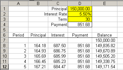
The yellow cells are user input cells. The Payment cell has this formula
=-ROUND(PMT(D2/12,D3*12,D1),2)
Because I am using a positive present value in the PMT() function, I negate the whole function to return a positive payment.
Period I just filled a series of numbers down to 360. You could make a formula for this, but I never do. If I wanted to make it dynamic, I would conditionally format the rows to make the text color the same as the background color if it exceeds the term.
Principal B8 =D8-C8
The interest and payment are calculated, so this column simply subtracts them.
Interest C8 =ROUND(E7*$D$2/12,2)
Multiply the loan balance by the interest rate divided by 12. The important thing to remember when building an amortization schedule is to keep your periods consistent. The payments are monthly, so the interest rate is converted to months. In the PMT() function above, the interest rate is also divided by12 and the nper (in years) is multiplied by 12.
Payment D8 =$D$4
That one’s pretty easy. I’ve computed the payment above and it doesn’t change, so I refer to that calculation.
Balance E8 =E7-B8
The old balance less the principal reduction for this payment. E7 refers to D1, the starting balance.
Now fill all these formulas down as far as you need. The ending balance probably won’t be zero. This is a pretty simplified amortization. The bank likes to complicate things with 360 day years and APR’s, but I like to keep it simple.
thanks you so much, just what I was looking for!
Thanks it has been a big help.
Thanks for the great table.
Your web site is a great find! Thanks for the very useful and easily understood information.
OWESOME< THANKS A TON
Thank you so much this was so helpful and saved us some extra $$ too!!!!
This post doesn’t add too much to Dick’s example but it does offer an opportunity to look at two of Excel’s lesser used financial functions.
While PMT is commonly used, its two sub-components, PPMT and IMPT, which find the principal and interest repectively in a given period aren’t as well known.
PMT = PPMT + IPMT
Principal in Period 1 = PPMT($D$2/12,A8,$D$3*12,$D$1)Interest in Period 1 = IPMT($D$2/12,A8,$D$3*12,$D$1)
and copy down
Cheers
Dave
I wanted to construct a simple speadsheet to illustrate what conditions would make a person become “upsidedown” in an auto loan. I used the 15% to 20% rule of thumb for annual depreciation. Presto! Illustates it quite well. Thanks!
I have never worked on Excel, but your example guided me through setting up an interest calculation spreadsheet very easily. Thanks so much!
Thanks a bunch! Saved lots of time and money! Well instructed!
I need help converting a spread sheet formula for a monthly payment into annual payments…
=IF(MONTH($A$10)>1,””,IF(MONTH($A$10)=1,ROUND($B$5*($D$5/1200),2),0))
I have this formula in my first column…How can I convert this thing to annually.
Thanks,
Kevin Box
If the term is 3 years, do you put 3 in the term or 36?
Very helpful.. Question though.
What if the balance is 125,000, interest rate is 5%, for 60 months and every month 1,000 is paid on the principle. How does this change the forumla and inputs??? Thanks
Does anyone have an amortization table that allows for missed payments and recapitalization of the missed interest?
If you just edit the payments (replace the formula with a dollar amount such as $0 for missed payments), it will recapitalize the interest.
if you could revise ur table to take care of situations where there is moratorium period before the amortization payment schedule takes effect.consider situations where interest charges does/does not accrue and whether the interst is coumpond or simple.
Thanks so much! This was very useful!!
Hi
This is helpful – but I am having trouble using the Excel functions based on a Daily interest rate..
for example £100,000 loan over 25 years at 5.5% using =-PMT(5.5/12,25*12,100000,0,0) gives the monthly payment of £614.09.
If I do this on a daily calc =-PMT(5.5/365,25*365,100000,0,0) gives a daily payment of £20.17. Now to make htis a monthly payment I multiply by 365 and divide by 12 I get £613.46.
OK this is not much of a difference but over the course of the loan of 300 payments this make a diference of £189.70 underpayment… good for mwe – but the bank will have a different view!!
Can any one suggest how to make this ballance out?
Thanks
GreenBoy
GreenBoy: F.I.s don’t do anything that lower their profits.
From what I can tell, you should “invert” your analysis.
First, calculate the FV at the appropriate rate.
Here’s a simple comparison. Calculate the total owed at the end of 1 year for a loan of 1 at a 10% annual rate.
With annual compounding, 1*(1+0.1)^1 = 1.1
With monthly compounding, 1*(1+0.1/12)^12 = 1.104713067
With daily compounding, 1*(1+0.1/365)^365 = 1.105155782
Next, calculate the payments. If their is only one payment to be made, it would be 1.1, 1.104713067, or 1.105155782 respectively. If they will be monthly, each would be 0.087540809, 0.087915887, or 0.08795112 respectively.
Greenboy,
You can’t sum up a componding function on a linear basis.
The reason for the “discrepancy” is that you are paying back the loan every day with the £20.17 payement – therefore the total interest payments to your lender are lower as your principal is smaller at the end of a month then the “montly loan”
Sounds good, but the flipside of course is that you have less funds to invest or conversely more to borrow to fund the faster loan payoff
Dave
Thanks , this table was a time and life saver
A typical amortization schedule is usually calculated for any type of loan that is for a specific amount to be paid off by a basic date in equal installments. You can use the amortization calculator to help you figure out the right mortgage for your home before you go and speak with a lender. Find more information and resources on my website.
free amortization.info
good day!
just wanna know why i arrive that answer in excel using ipmt function
i wanna ask for a formula how the excel calculated those data i entered
why excel arrive that answer.
thanx
To determine the best possible loan for your budget enter in different amounts into the amortization calculator to see what you will be able to afford. All of these types of amortization schedules are made to have a greater percentage of the payment going to interest as the loan starts out. Amortization is extremely important when it is time to make a decision on what mortgage company you should buy your home with in the long run. You can adjust the numbers in the amortization calculator to see if you will be able to make monthly payments on the loan amount you decide to borrow.
Hi
Has anyone come up with an example of how to build in a capital moratorium period / interest only option for say 12, 24 months into the loan amortisation?
========
if you could revise ur table to take care of situations where there is moratorium period before the amortization payment schedule takes effect.consider situations where interest charges does/does not accrue and whether the interst is coumpond or simple.
=======
would be grateful for any help.
thanks,
james
I need to determine what my ending balance is on a credit card after so many payments. So if I have a starting amount of $5,000 with an interest rate of 18% and a minimum monthly payment of $300 what would my balance be after 5 months/payment? How could I set this up in Excel? I don’t want to have to create an amortization table in order to do that. I just want to be able to enter in the values and get the result. I imagine it requires a macro with a loop, but if possible I would like a push in the right direction.
Thanks.
Brad:
Does anyone know of an Excel 2003 spreadsheet that caters for variable interest amounts.
For my home loan I have borrowed a specific amount over a specified time period and the interest rate is constantly changing.
I am making weekly repaymments greater than the minimum amount required.
Virtually all spreadsheets I have found are for a fixed interest rate. Could any of these be modified to accept a weekly interest rate figure ??
Any help appreciated
I think I was looking at this stuff too long. I had been playing with the FV function, but for some reason it didn’t register. Thanks for pointing out the obvious.
I need to keep track of payments for a piece of land sold but need to figure out interests on a daily basis. sometimes the payment is early or late, not always the same amout of money, and sometimes they skip a month.
Thanks in advance for you help.
John
I have pulled up your sight but it won’t let me erase any of your numbers to put mine in.
Very good tutorial. It always amazes me how a lot of people don’t seem to understand the mechanics of financial products. I run a mortgage information site myself and anything that can help to inform people and better equip them to understand how finance works is a good thing.
I am trying to work out how to do an amortisation table where the interest is not fixed for the entire period – it changes 1 year into the 15 year term. Can I still use the PMT function? If so, how do I input the data?
I am trying to work out how to do an amortisation table where the interest is not fixed for the entire period – it changes 1 year into the 15 year term. Can I still use the PMT function? If so, how do I input the data?
Someone please help. Here is my problem – 5 year loan @ 8% monthly payments are 2027.64. There were 26 loan payments made as of 5/23/07 and the prinicpal balance was $61,502.46 on that date. On June 8th 2007, 15 days later the loan was converted to stock in our company. I need the principal balance on June 8th! HELP I know the daily rat on the loan is .02192
$61,704.99
=FV(0.0002192,15,0,-61502.46)
I am new to excel but I posted the formula =-ROUND(PMT(D2/12,D3*12,D1),2) that was given out in 2004 for amortization/paymnet chart and it does not seem to work.
I am looking for a calulator somewhere on line or that i can develop in excel that will show accruing interest. My dilema is this: I gave loan with payment schedule to friend, but there have been many paymnets missing and at different intervals of time. How can I calculate this into a see a running balance of what is owed still with the interest accruing? thanks
Jim
Jim H,
You can do this using the IRR and Goal Seek functions. In the IRR function the first cell referred to will be your starting loan amount, and the remaining cells referred to will be the payments to date. Enter the starting amount as a positive number and the payments as negative or zeros. Be sure to include all the missed payments. The IRR function will then tell you the interest that you are actually earning to date.
You can then use Goal Seek on the final cell in the IRR formula to find out what your friend would have to pay to get back on track. If you want to figure multiple remaining payments, just set the extra ones equal to the one that you’re doing the Goal Seek on, in a formula, so that they all at once.
Because your friend has paid at different intervals your payment intervals in the IRR function might have to be very short, e.g., daily, in order to accurately figure the interest rate that has been paid to date, and the cells referenced in your formula will be mostly zeroes.
excellent example!
Thats owesome guys….!
u’v made my life easier in loan repayment calculations
Hi. I am trying to find/make a spreadsheet that will calculate savings in an investment account. I need something that allows for either weekly/fortnightly/monthly payments, but can calculate interest daily/weekly/monthly/yearly regardless of the frequency of the deposits. Can anyone help with this?
Hi this is haider trying to find a table to calculate the personal loan installments just input the loan amount tenur and rate that give me irr and the pmts and interest on monthly basis
thanks and regards
Hey this has been a great help!! Thank you so much…
Very nice, clear explanation! I need help calculating a monthly payment with interest accruing over a 365 day year. Can this be done with Excel formulas?
Brad: In cell A7, put the date the loan started (not the date of the first payment). In cell A8, put the date of the first payment. In A9:A?? put the dates of all the subsequent payments. Then in C8, your interest formula will be
and fill that down.
I’m searching for the right formula to determine payments on a loan with an interest-only period… i.e. 30 year loan, years 1-10 are interest only, then a rate of 7% applies for the remainder of the life of the loan. Thanks!
The FV part computes the present value argument to payment. It accrues interest on a $150k loan for 10 years at 7% with no payment. Then the PMT function handles the next 240 months.
Hi,
Eventhough i was little bit finance savy, I was facing little difficult to make amortisation table. I was always using standard one, which developed by some one.
It’s is very helpful.
Similar way, private banks are giving @ flat rate and still they say reducing balance. How to do that? Pl. help us
Regards,
Madhava
hi, can any body help me with the ammortization schedule which will calculate interest on daily basis.
I am trying to understand why my bank didn’t have the same payoff amount as me, and it looks like maybe it has something to do with the 360 day year and APR?? The payoff amount I had calculated was based off an Excel Amortization Table template from Microsoft. Can you explain the 360d day year and APR??
The 360 day year was invented back when bankers had to use abacuses. That is, it simplified the calculation. They kept it because they make slightly more money than with a 365 day year. 10% stated rate – 10%/365 = 0.02740% daily rate 10%/360 = 0.02778%
APR has to do with compounding. If I charge you 10% on a 1,000 loan, you would pay $100 in interest the first year if I compound annually. If I compound monthly, you pay
= $1,104.71 or 10.471% APR. That’s because in the second month, you’re paying interest on the interest you accrued in the first month (as well as the principle). In the third month, you’re paying interest on the interest you accrued in the first two months.
Daily on a 360 day year would be
= $1,105.16 or 10.516% APR
Sir or Madam,
Please direct me to a template that will add an insurance payment.
Thank you.
If you want to know more about “Create an Amortization Schedule in Excel”, check this link ……..
http://www.exceltip.com/excel-financial-formulas/create-an-amortization-schedule-in-microsoft-excel.html
Adding all the payments made leads to a total equal to the principle borrowed.
That can’t be right
Over the term of the loan, total payments made should be the principle plus interest accrued
Have i missed something?
Cancel that…my balance formula had the wrong cell
Thank you!!! very helpful!!! ive been scratching my head so bad
Please help me how to compute the Daily Payment basis and the terms to pay is up to 2 months period only and the interest rate for:
2 months term (60 days) is = 20%
1 and a half month (45 days) is = 15%
1 months (30 days) is = 10%
Take note i need a daily basis payment until he/she can paid the last day payment.